6 Model specification

suggests different analytic directions

6.1 Model specification based on a plot plan

The model employed to analyze corpus data must be related to the data structure. Nesting relationships have clear implications for model specification. Crossing, on the other hand, opens up the possibility of interaction patterns among factors. Interactions between predictor variables and factors belonging to the structural component (i.e. Speaker or Item) may also have implications for model specification, and may shed light on linguistically relevant variability in the data.

6.1.1 A plot plan for the ING data

Once the plot plan for a set of data is set up, with all structural and systematic components included, the nature of the different factors and their relationship can be directly translated into a model statement. An intermediate step is the transfer of the factors into the scheme shown in Figure Figure 6.1. The boxes in the middle tier feature the clustering factors (typically one or two) and the token-level predictors are listed at the bottom. The cluster-level predictors are written above their respective clustering factors. Figure Figure 6.2 shows the filled-in scheme for the (ING) data. Panel (a) gives a simplified version that ignores the clustering factor Item and the word-level predictors Word Class, Frequency, and Preceding Consonant. Panel (b) represents the full data layout.

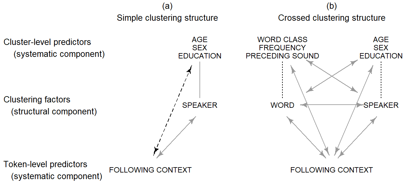
To start with, the model includes a term for each factor. All factors except the ones shown in boxes are fixed factors. The dotted lines extending from each box to its associated level-2 predictors represents a nesting relationship: Speakers are nested withing speaker-level predictors, and words are nested within word-level predictors. This nesting relationship is represented in the model if the Speaker and Item are specified as random factors.

The arrows in Figure Figure 6.2 show additional terms in the full model. Grey arrows denote crossing relationships involving a random factor. As we noted in Chapter Chapter 4, language-internal and -external clustering factors are crossed. Also, each clustering factor is crossed with any token-level predictor. Finally, each clustering factors is crossed with any level-2 predictors linked to another clustering factor. For instance, Speaker is crossed with any word-level predictor. Black arrows, on the other hand, indicate crossing relationships between fixed factors.

In principle, crossing relationship suggest the inclusion of interaction terms into the model. Interaction terms add complexity to a regression model, and it is in many cases unreasonable to represent all crossing relationship as interactions. However, the exclusion of interaction terms should proceed in an informed manner – we need to understand the consequences of a given reduction in model complexity. In Figure Figure 6.2 b, there are three different kinds of crossing relationship, which are shown with different types of arrows. These three types of crossing relationships require different treatment.

Crossing relationships between fixed factors are shown using black arrows. Whether an interaction between fixed factors should be part of the model depends on the researcher’s aims and background knowledge. The data layout provides no guidance. Note, however, that crossing relationships between level-2 and level-1 predictors are shown using dashed black arrows. Here, the plot plan does offer some guidelines, to which we will return shortly.

Grey arrows represent crossing relationships involving at least one random factor. Leaving out interaction terms of this type is appropriate only in certain fairly restricted situations. In general, if we decide to leave out one of these terms, it will be replaced by an additional modeling assumption, which can be considered as an additional requirement for valid statistical inferences. This means that the resulting inferences are meaningful only if these additional assumptions are approximately met by the data. All of these assumptions involve the idea of consistency – or constancy – of the pattern associated with a given factor. Let us first consider the crossing relationship between our clustering factors. Leaving out this interaction means that we are comfortable with the assumption that the systematic differences we observe between words will be consistent across speakers. Depending on the structure under study, this assumption will be more or less reasonable. If we are not comfortable with conditioning our inferences on the approximate truth of this assumption, we should include an interaction between Speaker and Item .

Next, consider the crossing relationship between the clustering factors, Speaker and Item, with each token-level predictor. Absence of interaction here implies that the token-level predictor in question behaves consistently across clusters. An interaction between Speaker and Following Consonant, for instance, signals that speakers react differently to coarticulatory constraints. Some speakers may show a more pronounced sensitivity to the articulatory context, others may show virtually no differences in the rate of g-dropping in different contexts. Similar considerations apply to Item.

6.1.2 Random intercepts and random slopes

The data layouts that call for an incorporation of random intercepts are different from those that suggest the addition of random slopes. The difference can be understood quite well when looking at our plot plan for corpus data. Random intercepts are needed if our data include predictors measured at the level of the subject or word. These are sometimes referred to as level-2 predictors. Random intercepts then basically inform the analysis about the appropriate sample size for these predictors. In general, then, if the data show clustering and there are cluster-level predictors, the model must include random intercepts.

In the literature on the design and analysis of experiments, this issue is treated under the notion of the experimental unit. Thus, a single experiment or study may include experimental units of different size. The design and execution of the experiment determine the size and number of experimental units associated with each factor in the analysis. For corpus data, the situation is simpler. We can rely on our understanding of the linguistic data setting. Instead of experimental unit, we use the term unit of analysis. Thus each predictor is tied to a certain unit of analysis. It is usually straightforward to identify the relevant unit of analysis for a predictor. [DoE: split plot designs. The name derives from its use in agriculture.]

Clusters are nested in the predictor.
Another setting: No predictors, but overall average.

The question of whether random slopes should be included in a model is relevant in different settings. This question comes up when there is a predictor that is crossed with subjects and/or words. Three types of crossing can occur:

Token-level predictors may be crossed with subjects and words
Word-level predictor can be cropssed with subjects
Subject-level predictors may be crossed with word

In such settings, we could, in principle, break down the data by subject/word and look at the the predictor for each subject/word individually. If we have enough data to do so, this would give us an idea of whether the association between predictor and outcome is stable across subjects and/or words. It would allow us to answer the question of how much variation we observe among speakers or words with respect to this predictor. We could express the relationship between predictor and outcome for each subject with a parameter, and then we could look at the distribution of these parameters. Ideally, all parameters are very similar, indicating that the predictor of interest operates similarly across speakers or words. As the variation between speakers or words grows, the average over these parameters becomes less and less representative of the set of units.

Our default attitude will be to consider the possibility that predictor parameters may vary across speakers and/or words. This means that we will always make an effort to inspect and understand this type of variability. Once we have looked at the distribution of parameters, we can decide how to proceed. Essentially, we have three options.

We could decide to ignore any variation that may exist between speakers and/or words. This simplifies our analysis and seems like a reasonable option if the variation among speakers is small. Our analysis then proceeds on the assumption that predictor parameters are constant across individuals/words, with observed variation being the result of sampling variation.

A second option would be to represent between-speaker variability in the predictor parameters in the form of random slopes. These enable the model to take into account the variation in parameter values across individuals. Statistical uncertainty estimates are adjusted accordingly. The model then returns a parameter that expresses the amount of between-subject variability.

A third option would be similar to the second one, but we add fixed rather than random slopes. This may be an option if our interest is focused on the specific units. This is probably more likely for words than for subjects.

The advice that is frequently offered in the statistical literature is to use a statistical test, or a model comparison, to decide whether there is heterogeneity in the parameter values and therefore whether this should be represented in the analysis. We should note that the significance criterion for such a test is usually more lenient, because rejecting the null hypothesis is usually not in the interest of the investigator (elaborate on this). Thus, p-values are set to .20 (Maxwell et al. 2017: 559) or .25 (Lawson 2015: 128). What appears to be problematic with this approach is that it relies exclusively on inferential criteria. If the statistical power of such test is low, this is problematic. We therefore prefer to address this issue descriptively, by appreciating the amount of variability that is there, relating it to the average predictor value across subjects, and then deciding how to proceed.

In experiments, randomization balances out the heterogeneity (Kish 1987: 13-14)
Heterogeneity of treatment effects
Unit-treatment additivity (Cox & Reid 2000)

6.1.3 Nested variables are treated as random factors

Nested variables that constitute part of the structural component, i.e. our clustering variables Speaker and Item, are typically treated as random effects. While this modeling strategy seems to be fairly uncontroversial for handling the factor Speaker, there are situations where it can be argued that Item may equally well be handled as a fixed effect. We will elaborate on this modeling decision further below. For now, we treat both factors as random, which is the preferred strategy when clustering variables are nested, and interest is focused on level-2 predictors measured on speakers (e.g. Age and Sex) and words (e.g. Word Class and Frequency).

By specifying nested structural factors as random effects, we build into the model the appropriate relationship between (i) Speaker and any speaker-level predictors and (ii) Item and any word-level predictors. This means that we clarify the unit of analysis for level-2 predictors.

6.1.4 Speaker-level predictors: Consequences of ignoring nesting

6.1.5 Token-level predictors

Due to this crossed relationship, the data provide information about systematic variability in g-dropping by Following Place of Articulation not just averaged across the 66 speakers, but also for each speaker individually. This is to say that we can assess, for each informant, how the share of /ɪŋ/-realizations varies over the four contexts. This will allow us to appraise the level of consistency across speakers. This consistency sheds light on the between-speaker stability of this articulatory constraint, and therefore nicely supplements the information that we obtain from averaging over the 66 speakers in our sample. It reveals to which extend the average pattern holds at the level of the individual speaker. The status of constraints that are relatively stable across speakers is different from those that fluctuate widely across speakers. These two perspectives, the aggregate and the person-specific level of description are combine features of the nomothetic (generalizing) and the idiographic (particularizing) approach to data analysis.

Looking at the token counts in the lower part of Figure Figure 4.8, there are quite a few sparsely populated cells, especially for velar contexts. Such cells are not going to provide us with reliable speaker-specific estimates. For coronal and other contexts, however, we observe relatively comfortable token counts. Data sparsity, then, can be an obstacle for the assessment of speaker-specific behavior. In such cases where token counts are too small to yield reliable estimates, the evaluation of between-speaker consistency can rely on summary measures of pattern stability, for instance in the form of a standard deviation parameter.

The crossing relationship between Item and Following Place of Articulation also allows us to investigate the variation in the likelihood of g-dropping across different phonetic contexts at different levels. Apart from calculating overall averages, we could look into this constraint at the level of the individual words. This will shed light on the differences among the words in terms of their susceptibility to the phonetic context. Between-word variation again addresses the question of consistency with which the constraint operates. However, our linguistic curiosity is likely to take us to the idiographic level of analysis. Thus, if certain words show a stable pronunciation across the four contexts, we would like to know which ones. Why do they run counter to the general trend in that they are largely unaffected by the following place of articulation? We would try to make sense of this finding, and our linguistic intuitions and experience may suggest different possible explanation. Perhaps lexical frequency plays a role, which could lead to stable, entrenched pronunciation routines. Or perhaps high-frequency strings show stronger phonetic fusion and assimilation (e.g. going to). In any case, between-word variability is likely to pose further questions and can lead to linguistic insights.

Data sparsity, of course, again is the bottleneck at the idiographic, lexeme-specific level of analysis. Given the ubiquity of Zipfian frequency profiles, it is not unlikely that the number of tokens available per lexical item quickly levels off into the single-digit range. This is evident from Figure ?fig-ing-following-context-crossed-with-item. Note that we have picked those words that occur at least 20 times. More then 700 words are not shown. Now, even though we are looking at the top end of the frequency list, there are quite a few empty cells. Reliable estimates for the conditions of interest are likely to emerge only for the top-frequency forms. We can fall back on summary measures of between-word variability, and enrich these with a reasonable selection of words.

Both crossing relationships afford the opportunity to study between-cluster consistency of token-level predictors, and – subject to the condition of sufficient tokens counts – to advance to an idiographic analysis perspective. This allows us to appreciate whether, and to what extent, average patterns materialize within clusters.

6.1.6 Token-level predictors: Bias

Whenever a multilevel model includes token-level predictors, there is the danger that the estimates for these predictors are biased. Bias may arise when there is an association between the token-level variable and a clustering variable. An association reflect difference among clusters in the distributinon of token-level variables. We will deal with such situations in Chapter ?sec-within-between.

6.2 Dealing with categorical units

The plot plan also makes clear when categorical units should and should not be removed from the data.

6.3 The function of random effects in data analysis

Statistical tools for addressing questions of generality
Statistical tools for studying patterns of variation
Intermediate position between the idiographic and nomothetic approach
Statistical tools for obtaining more accurate cluster-specific predictions

6.4 Consequences of model misspecification

As we will demonstrate shortly, this has implications for the analysis of within-subjects (our token-level) factors. In other settings, the blocking factor is not routinely considered as random. The analysis of a token-level predictor then depends on whether the pattern we observe for the token-level predictor is consistent across blocks (i.e. subjects). This means that the difference(s) of interest is (are) stable across blocks. We usually consult the data to decide whether consistency among subjects is a reasonable assumption to make.¹ If there is evidence of between-subject variation with regard to the difference of interest, the analysis proceeds along similar lines as when subject is treated as a random factor. The statistical uncertainty surrounding our key comparisons will then be wider.

¹ This is usually done via some preliminary test. The alpha-level for such tests is not the conventional .05, but usually set to .25 (cf. Bancroft (1964)) or .20. This threshold is given in various textbooks (e.g. Hinkelmann and Kempthorne (2008, 313); Lawson (2015, 128)); Maxwell, Delaney, and Kelley (2018, 559)).

Such decisions are best based on substantive grounds. Anderson (2001, 178) notes, for instance, that differences among subjects with regard to the difference of interest “may generally be taken for granted”.

If we are dealing with a token-level predictor crossed with subjects. Note that for token-level predictors, we do not usually talk about subsampling

6.4.1 Random intercepts and random slopes

(Rabe-Hesketh and Skrondal 2021, 214) note that because the correlation between intercept and slope depends on how x is scaled, it does not make sense to set the correlation to zero by specifying uncorrelated intercepts and slopes.

Interesting: (Rabe-Hesketh and Skrondal 2021, 235, 407) state that a model may include random slopes for a level-2 predictor to construct heteroskedastic random intercepts. (?)

6.5 Connection to other literatures

6.5.1 Connections to the DoE literature

The within-subject design corresponds to a randomized complete block design (RCBD). Usually, these are run with each speaker producing only a single replicate per token-level condition. In natural language use, we never obtain such balanced data situations. We routinely have, for most speakers, multiple tokens per token-level condition. Thus, the situation corresponds more closely to what is called a generalized randomized block design (GRBD). The way in which these design are analyzed depends on the nature of the blocking factor. In sciences studying human beings, it seems to be common to regard blocks (i.e. subjects) as random.²

² Apart from substantive considerations, which clearly point to subject as a random factor, there are very likely also practical reasons for this choice. Thus, in psychological studies, it is easy to have a comfortably high number of subjects. The number of levels of the blocking factor can therefore easily be as large as 30, say. In other disciplines, the number of blocks is more restricted. This is the case, for instance, in agricultural work. This may partly explain the readiness of psychological researchers to consider the blocking factor as random.

6.5.2 Agriculture vs. language sciences: Mapping issues

One problem is the notion of a replicate for the common layout of a strip-plot or strip-plot design. In agricultural experiments, all whole-plot units are units are perfectly replicable. In language data, if we define the whole-units to be speakers or words, these are not replicable in the same way. A second replicate of the whole-unit factor gender would involve two new speakers. This is not problem, in principle. But if we are looking at strip-plot layouts, with words as a second type of whole-unit, a replicate would also involve a second set of new words. And this is not what is happening.

It therefore seems that we need to conceptualize our plot plan ina different way. The basic point of the notion of replicates (and top-level blocks) is to use the appropriate error term for comparisons of whole-plot factors. For natural language data, determine the unit of analysis for different factors does not seem to be too difficult. So what we can do instead in our plot plan is to merge the different speakers and words into one array, and then annotate our speaker-and word-level predictors at the margins.

The fact that we are not dealing with top-level blocks means that the “design” for speaker- and word-level predictors changes slightly. In the split-plot and strip-plot literature, these error terms are always based on a randomized complete block design, because the whole-plot factors are replicated within blocks. Therefore, the error term is the Block x Factor interaction, which is typical for this type of design. In our modified arrangement we are looking at the equivalent of a completely randomized design. The error term is therefore a slightly different one.