Conditional vs. standard variable importance in random forests

corpus linguistics

bias

binary data

random forests

In this blog post, I demonstrate the differences between conditional and standard variable importance measures for random-forest models.

Author

Affiliation

Lukas Sönning

University of Bamberg

Published

April 13, 2026

R setup

library(party)
library(permimp)
library(lattice)
library(vcdExtra)
library(tidyverse)
library(ggthemes)
library(uls)

library(rethinking)
library(dagitty)

set.seed(1985)

For researchers working with random-forest models, it is critical to be aware of the difference between standard and conditional variable importance measures. In this blog post, I use simulated data to illustrate how these two types of scores respond to the presence of associations between predictor variables and interactions between predictor variables.

In our simulated set of data, there are two predictors, X and C, and an outcome variable Y. I will distinguish between two causal scenarios, which are shown using DAGS in the figure below:

Scenario 1: Confounding. Both predictors have a direct causal effect on Y, but C also causally affects X. C is therefore a confounder. This causal constellation is shown in the left DAG.
Scenario 2: No confounding. Both predictors have a direct causal effect on Y, and there is no causal relationship between X and C. This constellation is shown in the right DAG.

draw DAG

dag_conf <- dagitty( "dag{X -> Y;
                         C -> X; 
                         C -> Y}")

coordinates(dag_conf) <- list(
  x=c(X = 0, C = 1, Y = 2),
  y=c(X = 1, Y = 1, C = 0)
)

dag_no_conf <- dagitty( "dag{X -> Y; 
                         C -> Y}")

coordinates(dag_no_conf) <- list(
  x=c(X = 0, C = 1, Y = 2),
  y=c(X = 1, Y = 1, C = 0)
)

par(mfrow = c(1, 2))
drawdag(dag_conf, xlim = c(-.5,2.5))
drawdag(dag_no_conf, xlim = c(-.5,2.5))
par(mfrow = c(1, 1))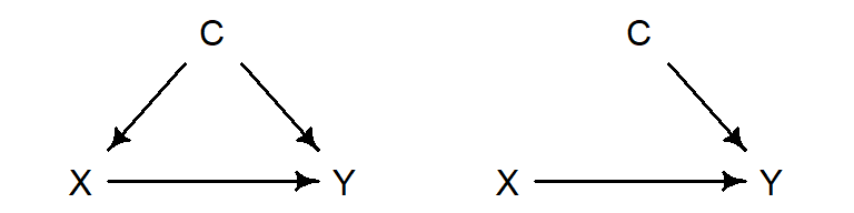

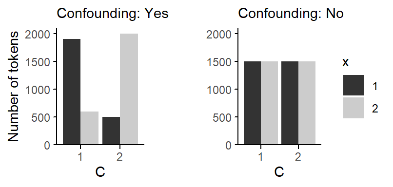
Figure 1: Directed acyclic graph for the simulated dataset.

If there is a causal effect of C on X, there will be an association between the two variables. This is illustrated in the bar chart below. In the left panel, the distribution of X varies with C, which reflects the causal effect C has on X. In the right panel, the two variables are independent – the distribution of X is the same for both levels of C.

The second feature we will vary is whether or not there is an interaction between X and C. Note that this question is independent of the question of whether there is confounding. In the line plots below, an interaction is reflected in non-parallel lines.

The final feature we will vary is whether X has a main effect.

The data we simulate include two additional predictors that represent noise: A binary one (random_binary) and a continuous one (random_continuous). The purpose of these additional, inert factors is that they make random-forest modeling, which involves predictor sampling, more feasible. In addition, the importance scores for these features provides a baseline.

Scenario 1: No confounding

Scenario 1a: Interaction, no X main effect

simulate data

d <- data.frame(
  x    = c(1,2, 1,2),
  conf = c(2,2, 1,1),
  prop = c(.65, .55, .35, .45),
  n    = c(1500, 1500, 1500, 1500)
)

d$y_0 <- d$n - d$n*d$prop
d$y_1 <- d$n*d$prop

d1 <- d |> gather(y_0:y_1, key = "variant", value = "Freq")

d1 <- vcdExtra::expand.dft(d1)

d1$y <- ifelse(d1$variant == "y_1", 1, 0)

d1$x <- factor(d1$x)
d1$conf <- factor(d1$conf)

d1$random_binary <- factor(rbinom(nrow(d1), size = 1, prob = .5))
d1$random_continuous <- rnorm(nrow(d1), mean = 0, sd = 1)
d1$y_factor <- factor(d1$y)

d1a <- d1

draw figure

d1a |> ggplot(aes(x = x, y = prop, group = conf, color = conf)) +
  geom_point(aes(size = n), bg = "white") +
  geom_line() +
  scale_size_area() +
  labs(subtitle = "Confounding: No\nInteraction: Yes\nMain effect of X: No") +
  theme_classic_ls() +
  scale_color_grey() +
  theme(legend.position = "none") +
  scale_y_continuous(limits = c(0,1), expand = c(0,0),
                     breaks = c(0,.5,1), label = c("0", ".5", "1")) +
  annotate("text", x = 2.3, y = c(.65, .45), label = c("C1", "C2"), adj=0) +
  ylab("Proportion")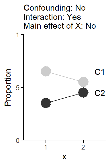

rf1a <- party::cforest(
  y_factor ~ x + conf + random_binary + random_continuous, 
  control = party::cforest_unbiased(
    mtry = 2, 
    ntree = 500), 
  d1a)

calculate VIMs

varimp_rf1a_cnd <- permimp::permimp(
  rf1a,
  conditional = TRUE,
  progressBar = FALSE)$values

varimp_rf1a_cnd <- as.data.frame(varimp_rf1a_cnd)
varimp_rf1a_cnd$variable <- rownames(varimp_rf1a_cnd)


varimp_rf1a_std <- permimp::permimp(
  rf1a,
  conditional = FALSE,
  progressBar = FALSE)$values

varimp_rf1a_std <- as.data.frame(varimp_rf1a_std)
varimp_rf1a_std$variable <- rownames(varimp_rf1a_std)

saveRDS(varimp_rf1a_cnd, "C:/Users/ba4rh5/Work Folders/My Files/R projects/_lsoenning.github.io/posts/2026-04-13_rfs_conditional_standard_vim/varimp_rf1a_cnd.rds")
saveRDS(varimp_rf1a_std, "C:/Users/ba4rh5/Work Folders/My Files/R projects/_lsoenning.github.io/posts/2026-04-13_rfs_conditional_standard_vim/varimp_rf1a_std.rds")

draw figure

varimp_rf1a_cnd |> 
  ggplot(aes(x = varimp_rf1a_cnd,
             y = variable)) +
  geom_col() +
  ylab(NULL) +
  xlab("Conditional variable importance") +
  labs(subtitle = "Confounding: No\nInteraction: Yes\nMain effect of X: No")

draw figure

varimp_rf1a_std |> 
  ggplot(aes(x = varimp_rf1a_std,
             y = variable)) +
  geom_col() +
  ylab(NULL) +
  xlab("Standard variable importance") +
  labs(subtitle = "Confounding: No\nInteraction: Yes\nMain effect of X: No")

Scenario 1b: Interaction, X main effect

simulate data

d <- data.frame(
  x    = c(1,2, 1,2),
  conf = c(2,2, 1,1),
  prop = c(.65, .60, .35, .50),
  n    = c(1500, 1500, 1500, 1500)
)

d$y_0 <- d$n - d$n*d$prop
d$y_1 <- d$n*d$prop

d1 <- d |> gather(y_0:y_1, key = "variant", value = "Freq")

d1 <- vcdExtra::expand.dft(d1)

d1$y <- ifelse(d1$variant == "y_1", 1, 0)

d1$x <- factor(d1$x)
d1$conf <- factor(d1$conf)

d1$random_binary <- factor(rbinom(nrow(d1), size = 1, prob = .5))
d1$random_continuous <- rnorm(nrow(d1), mean = 0, sd = 1)
d1$y_factor <- factor(d1$y)

d1b <- d1

draw figure

d1b |> ggplot(aes(x = x, y = prop, group = conf, color = conf)) +
  geom_point(aes(size = n), bg = "white") +
  geom_line() +
  scale_size_area() +
  labs(subtitle = "Confounding: No\nInteraction: Yes\nMain effect of X: Yes") +
  theme_classic_ls() +
  scale_color_grey() +
  theme(legend.position = "none") +
  scale_y_continuous(limits = c(0,1), expand = c(0,0),
                     breaks = c(0,.5,1), label = c("0", ".5", "1")) +
  annotate("text", x = 2.3, y = c(.65, .45), label = c("C1", "C2"), adj=0) +
  ylab("Proportion")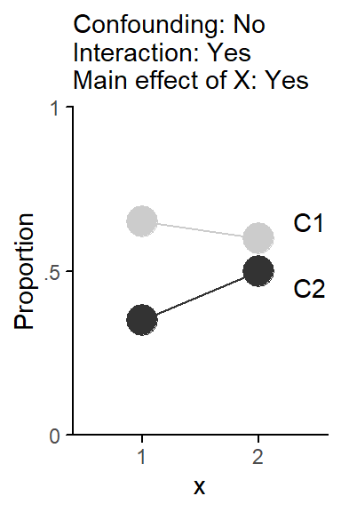

rf1b <- party::cforest(
  y_factor ~ x + conf + random_binary + random_continuous, 
  control = party::cforest_unbiased(
    mtry = 2, 
    ntree = 500), 
  d1b)

calculate VIMs

varimp_rf1b_cnd <- permimp::permimp(
  rf1b,
  conditional = TRUE,
  progressBar = FALSE)$values

varimp_rf1b_cnd <- as.data.frame(varimp_rf1b_cnd)
varimp_rf1b_cnd$variable <- rownames(varimp_rf1b_cnd)


varimp_rf1b_std <- permimp::permimp(
  rf1b,
  conditional = FALSE,
  progressBar = FALSE)$values

varimp_rf1b_std <- as.data.frame(varimp_rf1b_std)
varimp_rf1b_std$variable <- rownames(varimp_rf1b_std)

saveRDS(varimp_rf1b_cnd, "C:/Users/ba4rh5/Work Folders/My Files/R projects/_lsoenning.github.io/posts/2026-04-13_rfs_conditional_standard_vim/varimp_rf1b_cnd.rds")
saveRDS(varimp_rf1b_std, "C:/Users/ba4rh5/Work Folders/My Files/R projects/_lsoenning.github.io/posts/2026-04-13_rfs_conditional_standard_vim/varimp_rf1b_std.rds")

draw figure

varimp_rf1b_cnd |> 
  ggplot(aes(x = varimp_rf1b_cnd,
             y = variable)) +
  geom_col() +
  ylab(NULL) +
  xlab("Conditional variable importance") +
  labs(subtitle = "Confounding: No\nInteraction: Yes\nMain effect of X: Yes")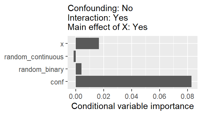

draw figure

varimp_rf1b_std |> 
  ggplot(aes(x = varimp_rf1b_std,
             y = variable)) +
  geom_col() +
  ylab(NULL) +
  xlab("Standard variable importance") +
  labs(subtitle = "Confounding: No\nInteraction: Yes\nMain effect of X: Yes")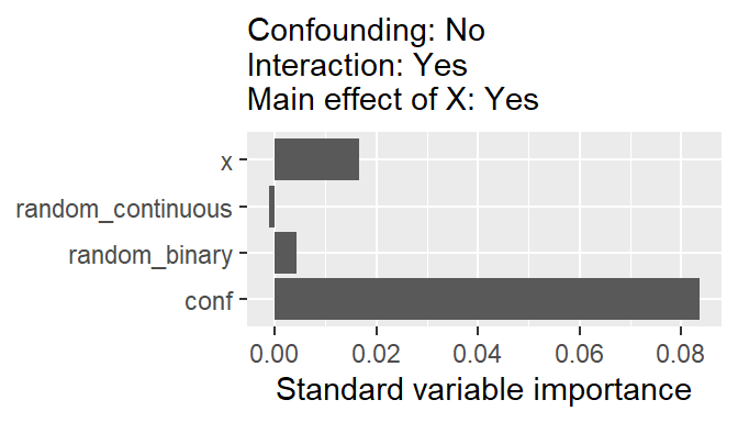

Scenario 1c: No interaction, X main effect

simulate data

d <- data.frame(
  x    = c(1,2, 1,2),
  conf = c(2,2, 1,1),
  prop = c(.6, .65, .4, .45),
  n    = c(1500, 1500, 1500, 1500)
)

d$y_0 <- d$n - d$n*d$prop
d$y_1 <- d$n*d$prop

d1 <- d |> gather(y_0:y_1, key = "variant", value = "Freq")

d1 <- vcdExtra::expand.dft(d1)

d1$y <- ifelse(d1$variant == "y_1", 1, 0)

d1$x <- factor(d1$x)
d1$conf <- factor(d1$conf)

d1$random_binary <- factor(rbinom(nrow(d1), size = 1, prob = .5))
d1$random_continuous <- rnorm(nrow(d1), mean = 0, sd = 1)
d1$y_factor <- factor(d1$y)

d1c <- d1

draw figure

d1c |> ggplot(aes(x = x, y = prop, group = conf, color = conf)) +
  geom_point(aes(size = n), bg = "white") +
  geom_line() +
  scale_size_area() +
  labs(subtitle = "Confounding: No\nInteraction: No\nMain effect of X: Yes") +
  theme_classic_ls() +
  scale_color_grey() +
  theme(legend.position = "none") +
  scale_y_continuous(limits = c(0,1), expand = c(0,0),
                     breaks = c(0,.5,1), label = c("0", ".5", "1")) +
  annotate("text", x = 2.3, y = c(.65, .45), label = c("C1", "C2"), adj=0) +
  ylab("Proportion")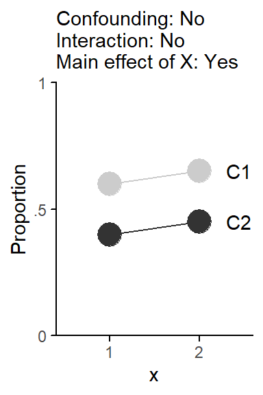

rf1c <- party::cforest(
  y_factor ~ x + conf + random_binary + random_continuous, 
  control = party::cforest_unbiased(
    mtry = 2, 
    ntree = 500), 
  d1c)

calculate VIMs

varimp_rf1c_cnd <- permimp::permimp(
  rf1c,
  conditional = TRUE,
  progressBar = FALSE)$values

varimp_rf1c_cnd <- as.data.frame(varimp_rf1c_cnd)
varimp_rf1c_cnd$variable <- rownames(varimp_rf1c_cnd)


varimp_rf1c_std <- permimp::permimp(
  rf1c,
  conditional = FALSE,
  progressBar = FALSE)$values

varimp_rf1c_std <- as.data.frame(varimp_rf1c_std)
varimp_rf1c_std$variable <- rownames(varimp_rf1c_std)

saveRDS(varimp_rf1c_cnd, "C:/Users/ba4rh5/Work Folders/My Files/R projects/_lsoenning.github.io/posts/2026-04-13_rfs_conditional_standard_vim/varimp_rf1c_cnd.rds")
saveRDS(varimp_rf1c_std, "C:/Users/ba4rh5/Work Folders/My Files/R projects/_lsoenning.github.io/posts/2026-04-13_rfs_conditional_standard_vim/varimp_rf1c_std.rds")

draw figure

varimp_rf1c_cnd |> 
  ggplot(aes(x = varimp_rf1c_cnd,
             y = variable)) +
  geom_col() +
  ylab(NULL) +
  xlab("Conditional variable importance") +
  labs(subtitle = "Confounding: No\nInteraction: No\nMain effect of X: Yes")

draw figure

varimp_rf1c_std |> 
  ggplot(aes(x = varimp_rf1c_std,
             y = variable)) +
  geom_col() +
  ylab(NULL) +
  xlab("Standard variable importance") +
  labs(subtitle = "Confounding: No\nInteraction: No\nMain effect of X: Yes")

Scenario 1d: No interaction, no X main effect

simulate data

d <- data.frame(
  x    = c(1,2, 1,2),
  conf = c(2,2, 1,1),
  prop = c(.6, .6, .4, .4),
  n    = c(1500, 1500, 1500, 1500)
)

d$y_0 <- d$n - d$n*d$prop
d$y_1 <- d$n*d$prop

d1 <- d |> gather(y_0:y_1, key = "variant", value = "Freq")

d1 <- vcdExtra::expand.dft(d1)

d1$y <- ifelse(d1$variant == "y_1", 1, 0)

d1$x <- factor(d1$x)
d1$conf <- factor(d1$conf)

d1$random_binary <- factor(rbinom(nrow(d1), size = 1, prob = .5))
d1$random_continuous <- rnorm(nrow(d1), mean = 0, sd = 1)
d1$y_factor <- factor(d1$y)

d1d <- d1

draw figure

d1d |> ggplot(aes(x = x, y = prop, group = conf, color = conf)) +
  geom_point(aes(size = n), bg = "white") +
  geom_line() +
  scale_size_area() +
  labs(subtitle = "Confounding: No\nInteraction: No\nMain effect of X: No") +
  theme_classic_ls() +
  scale_color_grey() +
  theme(legend.position = "none") +
  scale_y_continuous(limits = c(0,1), expand = c(0,0),
                     breaks = c(0,.5,1), label = c("0", ".5", "1")) +
  annotate("text", x = 2.3, y = c(.65, .45), label = c("C1", "C2"), adj=0) +
  ylab("Proportion")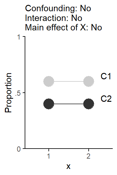

rf1d <- party::cforest(
  y_factor ~ x + conf + random_binary + random_continuous, 
  control = party::cforest_unbiased(
    mtry = 2, 
    ntree = 500), 
  d1d)

calculate VIMs

varimp_rf1d_cnd <- permimp::permimp(
  rf1d,
  conditional = TRUE,
  progressBar = FALSE)$values

varimp_rf1d_cnd <- as.data.frame(varimp_rf1d_cnd)
varimp_rf1d_cnd$variable <- rownames(varimp_rf1d_cnd)


varimp_rf1d_std <- permimp::permimp(
  rf1d,
  conditional = FALSE,
  progressBar = FALSE)$values

varimp_rf1d_std <- as.data.frame(varimp_rf1d_std)
varimp_rf1d_std$variable <- rownames(varimp_rf1d_std)

saveRDS(varimp_rf1d_cnd, "C:/Users/ba4rh5/Work Folders/My Files/R projects/_lsoenning.github.io/posts/2026-04-13_rfs_conditional_standard_vim/varimp_rf1d_cnd.rds")
saveRDS(varimp_rf1d_std, "C:/Users/ba4rh5/Work Folders/My Files/R projects/_lsoenning.github.io/posts/2026-04-13_rfs_conditional_standard_vim/varimp_rf1d_std.rds")

draw figure

varimp_rf1d_cnd |> 
  ggplot(aes(x = varimp_rf1d_cnd,
             y = variable)) +
  geom_col() +
  ylab(NULL) +
  xlab("Conditional variable importance") +
  labs(subtitle = "Confounding: No\nInteraction: No\nMain effect of X: No")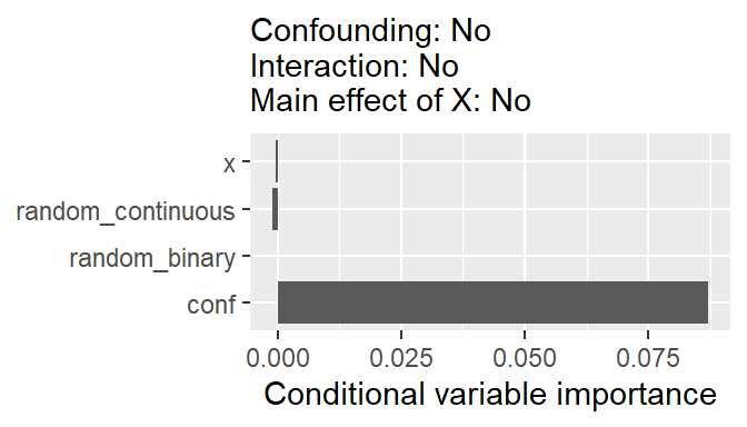

draw figure

varimp_rf1d_std |> 
  ggplot(aes(x = varimp_rf1d_std,
             y = variable)) +
  geom_col() +
  ylab(NULL) +
  xlab("Standard variable importance") +
  labs(subtitle = "Confounding: No\nInteraction: No\nMain effect of X: No")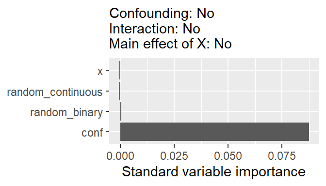

Scenario 2: Confounding

Scenario 2a: Interaction, no X main effect

simulate data

d <- data.frame(
  x    = c(1,2, 1,2),
  conf = c(2,2, 1,1),
  prop = c(.65, .55, .35, .45),
  n    = c(500, 2000, 1900, 600)
)

d$y_0 <- d$n - d$n*d$prop
d$y_1 <- d$n*d$prop

d1 <- d |> gather(y_0:y_1, key = "variant", value = "Freq")

d1 <- vcdExtra::expand.dft(d1)

d1$y <- ifelse(d1$variant == "y_1", 1, 0)

d1$random_binary <- factor(rbinom(nrow(d1), size = 1, prob = .5))
d1$random_continuous <- rnorm(nrow(d1), mean = 0, sd = 1)
d1$y_factor <- factor(d1$y)

d1$x <- factor(d1$x)
d1$conf <- factor(d1$conf)

d2a <- d1

draw figure

d2a |> ggplot(aes(x = x, y = prop, group = conf, color = conf)) +
  geom_point(aes(size = n), bg = "white") +
  geom_line() +
  scale_size_area() +
  labs(subtitle = "Confounding: Yes\nInteraction: Yes\nMain effect of X: No") +
  theme_classic_ls() +
  scale_color_grey() +
  theme(legend.position = "none") +
  scale_y_continuous(limits = c(0,1), expand = c(0,0),
                     breaks = c(0,.5,1), label = c("0", ".5", "1")) +
  annotate("text", x = 2.3, y = c(.65, .45), label = c("C1", "C2"), adj=0) +
  ylab("Proportion")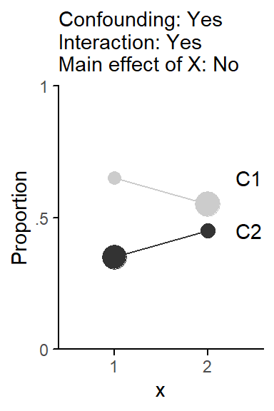

rf2a <- party::cforest(
  y_factor ~ x + conf + random_binary + random_continuous, 
  control = party::cforest_unbiased(
    mtry = 2, 
    ntree = 500), 
  d2a)

calculate VIMs

varimp_rf2a_cnd <- permimp::permimp(
  rf2a,
  conditional = TRUE,
  progressBar = FALSE)$values

varimp_rf2a_cnd <- as.data.frame(varimp_rf2a_cnd)
varimp_rf2a_cnd$variable <- rownames(varimp_rf2a_cnd)


varimp_rf2a_std <- permimp::permimp(
  rf2a,
  conditional = FALSE,
  progressBar = FALSE)$values

varimp_rf2a_std <- as.data.frame(varimp_rf2a_std)
varimp_rf2a_std$variable <- rownames(varimp_rf2a_std)

saveRDS(varimp_rf2a_cnd, "C:/Users/ba4rh5/Work Folders/My Files/R projects/_lsoenning.github.io/posts/2026-04-13_rfs_conditional_standard_vim/varimp_rf2a_cnd.rds")
saveRDS(varimp_rf2a_std, "C:/Users/ba4rh5/Work Folders/My Files/R projects/_lsoenning.github.io/posts/2026-04-13_rfs_conditional_standard_vim/varimp_rf2a_std.rds")

draw figure

varimp_rf2a_cnd |> 
  ggplot(aes(x = varimp_rf2a_cnd,
             y = variable)) +
  geom_col() +
  ylab(NULL) +
  xlab("Conditional variable importance") +
  labs(subtitle = "Confounding: Yes\nInteraction: Yes\nMain effect of X: No")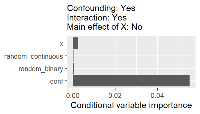

draw figure

varimp_rf2a_std |> 
  ggplot(aes(x = varimp_rf2a_std,
             y = variable)) +
  geom_col() +
  ylab(NULL) +
  xlab("Standard variable importance") +
  labs(subtitle = "Confounding: Yes\nInteraction: Yes\nMain effect of X: No")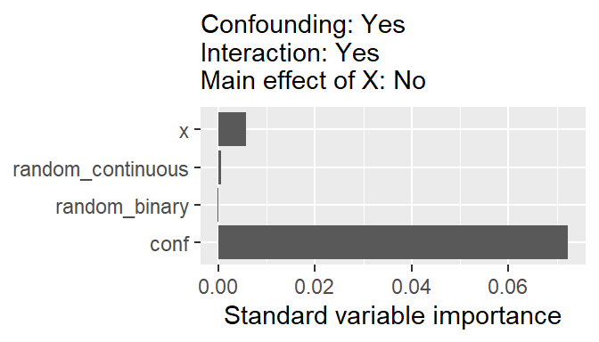

Scenario 2b: Interaction, X main effect

simulate data

d <- data.frame(
  x    = c(1,2, 1,2),
  conf = c(2,2, 1,1),
  prop = c(.65, .60, .35, .50),
  n    = c(500, 2000, 1900, 600)
)

d$y_0 <- d$n - d$n*d$prop
d$y_1 <- d$n*d$prop



d1 <- d |> gather(y_0:y_1, key = "variant", value = "Freq")

d1 <- vcdExtra::expand.dft(d1)

d1$y <- ifelse(d1$variant == "y_1", 1, 0)
d1$x <- factor(d1$x)
d1$conf <- factor(d1$conf)

d1$random_binary <- factor(rbinom(nrow(d1), size = 1, prob = .5))
d1$random_continuous <- rnorm(nrow(d1), mean = 0, sd = 1)
d1$y_factor <- factor(d1$y)

d2b <- d1

draw figure

d2b |> ggplot(aes(x = x, y = prop, group = conf, color = conf)) +
  geom_point(aes(size = n), bg = "white") +
  geom_line() +
  scale_size_area() +
  labs(subtitle = "Confounding: Yes\nInteraction: Yes\nMain effect of X: Yes") +
  theme_classic_ls() +
  scale_color_grey() +
  theme(legend.position = "none") +
  scale_y_continuous(limits = c(0,1), expand = c(0,0),
                     breaks = c(0,.5,1), label = c("0", ".5", "1")) +
  annotate("text", x = 2.3, y = c(.65, .45), label = c("C1", "C2"), adj=0) +
  ylab("Proportion")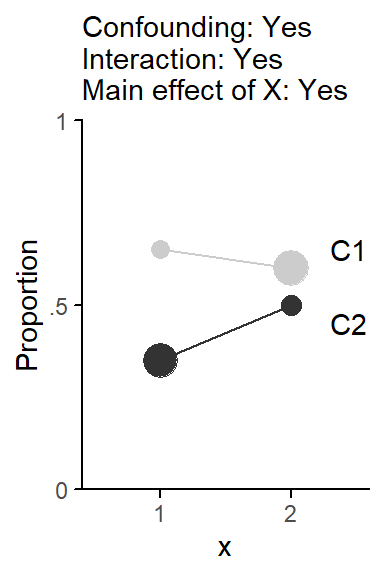

rf2b <- party::cforest(
  y_factor ~ x + conf + random_binary + random_continuous, 
  control = party::cforest_unbiased(
    mtry = 2, 
    ntree = 500), 
  d2b)

calculate VIMs

varimp_rf2b_cnd <- permimp::permimp(
  rf2b,
  conditional = TRUE,
  progressBar = FALSE)$values

varimp_rf2b_cnd <- as.data.frame(varimp_rf2b_cnd)
varimp_rf2b_cnd$variable <- rownames(varimp_rf2b_cnd)


varimp_rf2b_std <- permimp::permimp(
  rf2b,
  conditional = FALSE,
  progressBar = FALSE)$values

varimp_rf2b_std <- as.data.frame(varimp_rf2b_std)
varimp_rf2b_std$variable <- rownames(varimp_rf2b_std)

saveRDS(varimp_rf2b_cnd, "C:/Users/ba4rh5/Work Folders/My Files/R projects/_lsoenning.github.io/posts/2026-04-13_rfs_conditional_standard_vim/varimp_rf2b_cnd.rds")
saveRDS(varimp_rf2b_std, "C:/Users/ba4rh5/Work Folders/My Files/R projects/_lsoenning.github.io/posts/2026-04-13_rfs_conditional_standard_vim/varimp_rf2b_std.rds")

draw figure

varimp_rf2b_cnd |> 
  ggplot(aes(x = varimp_rf2b_cnd,
             y = variable)) +
  geom_col() +
  ylab(NULL) +
  xlab("Conditional variable importance") +
  labs(subtitle = "Confounding: Yes\nInteraction: Yes\nMain effect of X: Yes")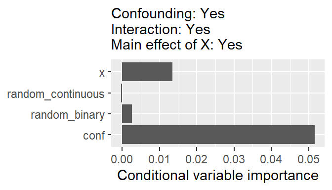

draw figure

varimp_rf2b_std |> 
  ggplot(aes(x = varimp_rf2b_std,
             y = variable)) +
  geom_col() +
  ylab(NULL) +
  xlab("Standard variable importance") +
  labs(subtitle = "Confounding: Yes\nInteraction: Yes\nMain effect of X: Yes")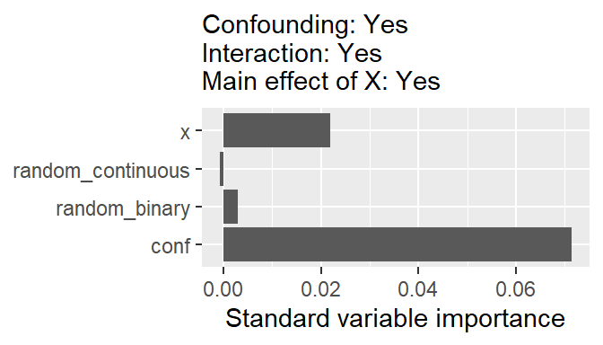

Scenario 2c: No interaction, X main effect

simulate data

d <- data.frame(
  x    = c(1,2, 1,2),
  conf = c(2,2, 1,1),
  prop = c(.6, .65, .4, .45),
  n    = c(500, 2000, 1900, 600)
)

d$y_0 <- d$n - d$n*d$prop
d$y_1 <- d$n*d$prop

d1 <- d |> gather(y_0:y_1, key = "variant", value = "Freq")

d1 <- vcdExtra::expand.dft(d1)

d1$y <- ifelse(d1$variant == "y_1", 1, 0)

d1$x <- factor(d1$x)
d1$conf <- factor(d1$conf)

d1$random_binary <- factor(rbinom(nrow(d1), size = 1, prob = .5))
d1$random_continuous <- rnorm(nrow(d1), mean = 0, sd = 1)
d1$y_factor <- factor(d1$y)

d2c <- d1

draw figure

d2c |> ggplot(aes(x = x, y = prop, group = conf, color = conf)) +
  geom_point(aes(size = n), bg = "white") +
  geom_line() +
  scale_size_area() +
  labs(subtitle = "Confounding: Yes\nInteraction: No\nMain effect of X: Yes") +
  theme_classic_ls() +
  scale_color_grey() +
  theme(legend.position = "none") +
  scale_y_continuous(limits = c(0,1), expand = c(0,0),
                     breaks = c(0,.5,1), label = c("0", ".5", "1")) +
  annotate("text", x = 2.3, y = c(.65, .45), label = c("C1", "C2"), adj=0) +
  ylab("Proportion")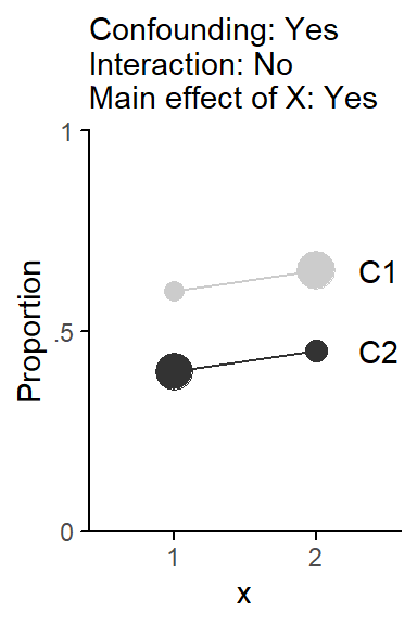

rf2c <- party::cforest(
  y_factor ~ x + conf + random_binary + random_continuous, 
  control = party::cforest_unbiased(
    mtry = 2, 
    ntree = 500), 
  d2c)

calculate VIMs

varimp_rf2c_cnd <- permimp::permimp(
  rf2c,
  conditional = TRUE,
  progressBar = FALSE)$values

varimp_rf2c_cnd <- as.data.frame(varimp_rf2c_cnd)
varimp_rf2c_cnd$variable <- rownames(varimp_rf2c_cnd)


varimp_rf2c_std <- permimp::permimp(
  rf2c,
  conditional = FALSE,
  progressBar = FALSE)$values

varimp_rf2c_std <- as.data.frame(varimp_rf2c_std)
varimp_rf2c_std$variable <- rownames(varimp_rf2c_std)

saveRDS(varimp_rf2c_cnd, "C:/Users/ba4rh5/Work Folders/My Files/R projects/_lsoenning.github.io/posts/2026-04-13_rfs_conditional_standard_vim/varimp_rf2c_cnd.rds")
saveRDS(varimp_rf2c_std, "C:/Users/ba4rh5/Work Folders/My Files/R projects/_lsoenning.github.io/posts/2026-04-13_rfs_conditional_standard_vim/varimp_rf2c_std.rds")

draw figure

varimp_rf2c_cnd |> 
  ggplot(aes(x = varimp_rf2c_cnd,
             y = variable)) +
  geom_col() +
  ylab(NULL) +
  xlab("Conditional variable importance") +
  labs(subtitle = "Confounding: Yes\nInteraction: No\nMain effect of X: Yes")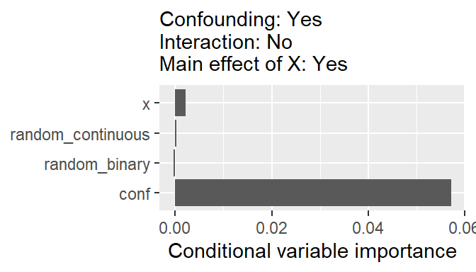

draw figure

varimp_rf2c_std |> 
  ggplot(aes(x = varimp_rf2c_std,
             y = variable)) +
  geom_col() +
  ylab(NULL) +
  xlab("Standard variable importance") +
  labs(subtitle = "Confounding: Yes\nInteraction: No\nMain effect of X: Yes")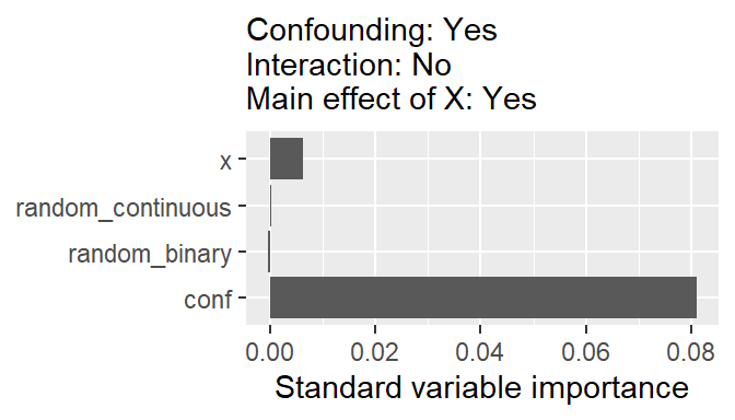

Scenario 2d: No interaction, no X main effect

simulate data

d <- data.frame(
  x    = c(1,2, 1,2),
  conf = c(2,2, 1,1),
  prop = c(.6, .6, .4, .4),
  n    = c(500, 2000, 1900, 600)
)

d$y_0 <- d$n - d$n*d$prop
d$y_1 <- d$n*d$prop

d1 <- d |> gather(y_0:y_1, key = "variant", value = "Freq")

d1 <- vcdExtra::expand.dft(d1)

d1$y <- ifelse(d1$variant == "y_1", 1, 0)

d1$x <- factor(d1$x)
d1$conf <- factor(d1$conf)

d1$random_binary <- factor(rbinom(nrow(d1), size = 1, prob = .5))
d1$random_continuous <- rnorm(nrow(d1), mean = 0, sd = 1)
d1$y_factor <- factor(d1$y)

d2d <- d1

draw figure

d2d |> ggplot(aes(x = x, y = prop, group = conf, color = conf)) +
  geom_point(aes(size = n), bg = "white") +
  geom_line() +
  scale_size_area() +
  labs(subtitle = "Confounding: Yes\nInteraction: No\nMain effect of X: No") +
  theme_classic_ls() +
  scale_color_grey() +
  theme(legend.position = "none") +
  scale_y_continuous(limits = c(0,1), expand = c(0,0),
                     breaks = c(0,.5,1), label = c("0", ".5", "1")) +
  annotate("text", x = 2.3, y = c(.65, .45), label = c("C1", "C2"), adj=0) +
  ylab("Proportion")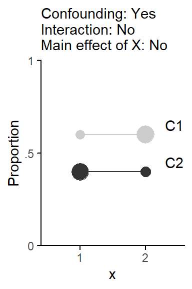

rf2d <- party::cforest(
  y_factor ~ x + conf + random_binary + random_continuous, 
  control = party::cforest_unbiased(
    mtry = 2, 
    ntree = 500), 
  d2d)

calculate VIMs

varimp_rf2d_cnd <- permimp::permimp(
  rf2d,
  conditional = TRUE,
  progressBar = FALSE)$values

varimp_rf2d_cnd <- as.data.frame(varimp_rf2d_cnd)
varimp_rf2d_cnd$variable <- rownames(varimp_rf2d_cnd)


varimp_rf2d_std <- permimp::permimp(
  rf2d,
  conditional = FALSE,
  progressBar = FALSE)$values

varimp_rf2d_std <- as.data.frame(varimp_rf2d_std)
varimp_rf2d_std$variable <- rownames(varimp_rf2d_std)

saveRDS(varimp_rf2d_cnd, "C:/Users/ba4rh5/Work Folders/My Files/R projects/_lsoenning.github.io/posts/2026-04-13_rfs_conditional_standard_vim/varimp_rf2d_cnd.rds")
saveRDS(varimp_rf2d_std, "C:/Users/ba4rh5/Work Folders/My Files/R projects/_lsoenning.github.io/posts/2026-04-13_rfs_conditional_standard_vim/varimp_rf2d_std.rds")

draw figure

varimp_rf2d_cnd |> 
  ggplot(aes(x = varimp_rf2d_cnd,
             y = variable)) +
  geom_col() +
  ylab(NULL) +
  xlab("Conditional variable importance") +
  labs(subtitle = "Confounding: Yes\nInteraction: No\nMain effect of X: No")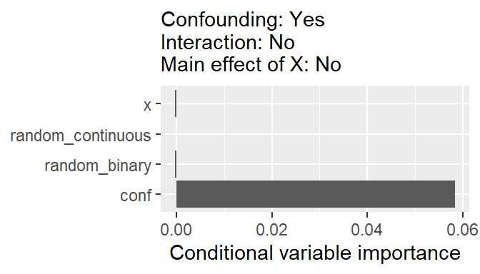

draw figure

varimp_rf2d_std |> 
  ggplot(aes(x = varimp_rf2d_std,
             y = variable)) +
  geom_col() +
  ylab(NULL) +
  xlab("Standard variable importance") +
  labs(subtitle = "Confounding: Yes\nInteraction: No\nMain effect of X: No")

In the first scenario, there is no interaction between C and X, which means that the effect of X does not vary across the levels of C. However, the association between X and C, which results from the causal effect of C on X (C -> X), is built into this simulation.

In a regression model without C, X has a spurious association with Y:

arm::display(
  glm(y ~ x + random_binary + random_continuous, 
      d1,
      family = "binomial")
)

glm(formula = y ~ x + random_binary + random_continuous, family = "binomial", 
    data = d1)
                  coef.est coef.se
(Intercept)       -0.23     0.05  
x2                 0.45     0.06  
random_binary1    -0.01     0.06  
random_continuous -0.03     0.03  
---
  n = 5000, k = 4
  residual deviance = 6867.5, null deviance = 6931.5 (difference = 63.9)

If we add C to the model, the association between X and Y goes to 0.

arm::display(
  glm(y ~ x + conf + random_binary + random_continuous, 
      d1,
      family = "binomial")
)

glm(formula = y ~ x + conf + random_binary + random_continuous, 
    family = "binomial", data = d1)
                  coef.est coef.se
(Intercept)       -0.41     0.05  
x2                 0.00     0.07  
conf2              0.81     0.07  
random_binary1     0.00     0.06  
random_continuous -0.03     0.03  
---
  n = 5000, k = 5
  residual deviance = 6729.0, null deviance = 6931.5 (difference = 202.5)

Citation

BibTeX citation:

@online{sönning2026,
  author = {Sönning, Lukas},
  title = {Conditional Vs. Standard Variable Importance in Random
    Forests},
  date = {2026-04-13},
  url = {https://lsoenning.github.io/posts/2026-04-13_random_forest_interaction_predictors/},
  langid = {en}
}

For attribution, please cite this work as:

Sönning, Lukas. 2026. “Conditional Vs. Standard Variable Importance in Random Forests.” April 13, 2026. https://lsoenning.github.io/posts/2026-04-13_random_forest_interaction_predictors/.