Issues in random-forest modeling: Interaction predictors

In this blog post, I demonstrate that the inclusion of manually specified interaction predictors into a random-forest model yields biased (or uninterpretable) partial dependence plots.

Author

Affiliation

Lukas Sönning

University of Bamberg

A practice that has emerged fairly recently in random-forest modeling is the inclusion of manually specified interaction predictors into RF models. Two motivations drive this approach: First, in the very unlikely situation where two predictors show no main effect but a perfect crossover interaction (referred to as the XOR problem), classification trees (and hence RF models) fail to recover the interaction. Further, variable importance scores derived from an RF model for a specific predictor conflate its main effect and its interaction effect(s). This means that variable importance scores, which are the most widespread method of interpretation for RF models, give no indication of the relative magnitude of these two types of effects.

These drawbacks have prompted the suggestion to manually specify interaction variables and include them into the RF model (Gries 2019, 638–40; see also Strobl, Malley, and Tutz 2009, 341). For two categorical predictors, for instance, an interaction predictor consists of the pairwise cross-combinations of all levels. For two binary variables – e.g. male/female and old/young – the interaction predictor would consist of four subgroups: male-young, male-old, female-young, female-old. Interaction predictors, it is argued, help shed light on the relative importance of interaction vs. main effects of predictors. I recently conducted a survey on the use of RF models in corpus research (Sönning 2026). In 8 out of 69 articles (12%) that applied an RF to corpus data, use was made of this modeling strategy, with the model including a manually specified interaction variable.

The recursive splitting algorithm operating under the hood of RF models handles interactions between predictor variables automatically. As such, RFs therefore have no problems detecting interactions (except for the case of the XOR problem mentioned above). The main motivation for including interaction variables, then, is to facilitate model interpretation.

In this blog post, I give two reasons why the practice of including interaction variables into a model is ill-advised. Contrary to the primary motivation behind including interaction predictors into a model, its interpretability actually suffers. This is for two reasons. The first concerns variable importance scores. As demonstrated by Strobl et al. (2024) using a simulation study, the importance attributed to an interaction predictor does not necessarily reflect the predictive importance of the interaction component. In fact, the interaction predictor will show spurious importance even if a statistical interaction is absent from the data. The second issue, which does not seem to have received much attention, concerns the construction and interpretation of partial dependence scores. I will show that, in the presence of both main effects and a statistical interaction between two variables, the partial dependence scores we construct from a model including an interaction predictor blend main effects an interaction effects and therefore fail to provide a clear picture of either form of relationship.

library(party)
library(permimp)
library(lattice)
library(vcdExtra)
library(tidyverse)
library(janitor)
library(uls)

Problem 1: Interaction variables are predictively important even when there is no interaction present

To demonstrate this issue, which was highlighted by Strobl et al. (2024), I will create some data that show no statistical interaction, neither on the scale of outcome proportions nor on the logit scale. Then I will fit a number of RF models to these data with different settings for the m_try parameter. For each of these models, I will then obtain two types of variable importance scores: standard and conditional importance scores.

Data

The data consist of 1,200 speakers, which are divided into four groups:

• 300 old, male
• 300 old, female
• 300 young, male
• 300 young, female

This means that there are two binary predictors, gender (male vs. female) and age (young vs. old). For some binary outcome variable of interest, these are the percentages in the four cells:

• 20% old, male
• 40% old, female
• 60% young, male
• 80% young, female

Figure 1 shows the structure we have built into the data.

# set seed for reproducibility
set.seed(123)

# number of observations per cell
n_obs_per_cell <- 300

# outcome proportions for each cell
probs <- c(.2, .4, .6, .8)

# simulate binary outcome
condition_were <- probs * n_obs_per_cell


d <- data.frame(
  #speaker = paste0("subj_", 1:n_speakers),
  age = c("old", "old", "young", "young"),
  gender = c("male", "female", "male", "female"),
  were = condition_were,
  was = n_obs_per_cell - condition_were
) |> 
  pivot_longer(
    cols = c("was", "were"), 
    names_to = "variant", 
    values_to = "freq")

d <- expand.dft(d, freq = "freq") 

d$age <- factor(d$age)
d$gender <- factor(d$gender)
d$variant <- factor(d$variant)
d$interaction <- factor(d$age:d$gender)
d$random_continuous <- rnorm(nrow(d))
d$random_binary <- rbinom(nrow(d), 1, .5)

d <- d[order(d$variant, decreasing = TRUE),]

d |> group_by(age, gender) |> 
  dplyr::summarize(
    mean_prop = mean(variant == "were")
  ) |> ggplot(aes(x = age, y = mean_prop, group = gender)) +
  geom_point() +
  scale_y_continuous(
    limits = c(0,1), expand = c(0,0),
    breaks = c(0, .5, 1),
    labels = c("0", ".5", "1")) +
  geom_line() +
  annotate("text", x = 2.1, y = c(.6, .8) + .02, 
           label = c("male", "female"),
           size = 3.2, adj = 0) +
  ylab("Proportion of interest") +
  xlab(NULL) +
  theme_classic_ls()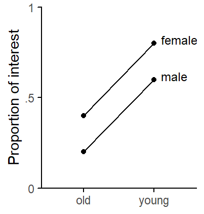

Figure 1: Line plot showing how the proportion of interest varies with age and gender.

We also add to the dataset two variables that represent random noise, a binary one (random_binary) and a continuous one (random_continuous). This is for two reasons:

• First, it will increase the number of predictors, making RF modeling (which includes predictor sampling) feasible
• Second, and more importantly, the variable importance scores we obtain for these noise variables are a useful point of reference for the predictors of interest. Due to the associations we have built into the model, age and gender should exceed both noise variables in predictive utility.

This is the dataset:

str(d)

tibble [1,200 × 6] (S3: tbl_df/tbl/data.frame)
 $ age              : Factor w/ 2 levels "old","young": 1 1 1 1 1 1 1 1 1 1 ...
 $ gender           : Factor w/ 2 levels "female","male": 2 2 2 2 2 2 2 2 2 2 ...
 $ variant          : Factor w/ 2 levels "was","were": 2 2 2 2 2 2 2 2 2 2 ...
 $ interaction      : Factor w/ 4 levels "old:female","old:male",..: 2 2 2 2 2 2 2 2 2 2 ...
 $ random_continuous: num [1:1200] -0.789 -0.502 1.496 -1.137 -0.179 ...
 $ random_binary    : int [1:1200] 0 1 0 0 1 1 1 0 1 0 ...

For reassurance, we check that the four cells reflect our intended percentages:

d |> tabyl(variant, gender, age) |> 
  adorn_percentages("col") |> 
  adorn_pct_formatting(digits = 0) |>
  adorn_ns()

$old
 variant    female      male
     was 60% (180) 80% (240)
    were 40% (120) 20%  (60)

$young
 variant    female      male
     was 20%  (60) 40% (120)
    were 80% (240) 60% (180)

Fit RF models and obtain variable importance scores

Next, I will fit a conditional random-forest model to these data using different settings for the m_try parameter. This parameter determines the number of predictor variables that are sampled at each splitting occasion during model fitting. I will let it vary from 2 to the total number of predictor variables (here: 5). If m_try equals the number of predictor variables, no predictor sampling takes place; this special case is referred to as bagging (Breiman 1996). For each RF model, I will then obtain two types of variable importance scores: standard and conditional importance scores.

The following simulation therefore varies two parameters:

• m_try parameter: 2, 3, 4, 5 predictors
• type of variable importance score: standard vs. conditional

set_mtry <- 2:5

sim_results <- array(
  NA, dim = c(5, 4, 2),
  dimnames = list(
    c("age", "gender", "interaction", "random_continuous", "random_binary"),
    set_mtry,
    c("conditional", "standard")))


for (i in 1:length(set_mtry)){
  
  # fit RF model
  rf <- party::cforest(
  variant ~ age + gender + interaction +
    random_continuous + random_binary, data = d,
      control = party::cforest_unbiased(
        mtry = set_mtry[i], 
        ntree = 1000))
  
  # obtain variable importance scores
  # conditional
  varimp_cond <- permimp(
    rf,
    conditional = TRUE,
    progressBar = FALSE)$values
  
  sim_results[,i,1] <- varimp_cond
  
  # standard
  varimp_std <- permimp(
    rf,
    conditional = FALSE,
    progressBar = FALSE)$values
  
  sim_results[,i,2] <- varimp_std

  }

sim_results_df <- as.data.frame(
  as.table(sim_results))

colnames(sim_results_df) <- c(
  "predictor", "mtry", "type", "score"
)

Comparison of importance scores

Figure 2 compares conditional variable importance scores (left panel) and standard variable importance scores (right panel) for different settings of the m_try parameter. The first observation that strikes us is that the interaction predictor always ranks first in terms of importance, despite the fact that the data show no statistical interaction (see Figure 1). While smaller values of the m_try parameter bring about some reduction in the importance of the interaction predictor, it always comes out on top. The predictive utility of age depends dramatically on the m_try parameter. In the case of bagging (m_try = 5), the predictor receives zero importance. The predictor gender, on the other hand, always hovers near zero. Standard and conditional variable importance score yield very similar picture, which is unsurprising seeing that we did not build into the data correlations among predictor variables.

sim_results_df$predictor <- factor(
  sim_results_df$predictor,
  levels = c("interaction", "age", "gender", "random_continuous", "random_binary"),
  ordered = TRUE
)

sim_results_df <- sim_results_df[order(sim_results_df$predictor, decreasing = TRUE),]

xyplot(
  1~1, type = "n", xlim = c(-.12, .35), ylim = c(-1, 7),
  par.settings = lattice_ls,
  scales = list(draw = FALSE),
  xlab = NULL, ylab = NULL,
  panel = function(x,y){
    panel.text(x = -.03, y = 1:5, label = c(
      "(Binary)", "(Continuous)", "Gender", "Age", "Interaction"), adj = 1, cex = .9)
    panel.segments(x0 = c(0, .2), x1 = c(0, .2), y0 = .3, y1 = 5.5, col = "grey")
    
    panel.points(x = subset(sim_results_df, mtry == "2" & type == "conditional")$score, 
                 y = 1:5, pch = "2", cex = 2.2)
    panel.points(x = subset(sim_results_df, mtry == "3" & type == "conditional")$score, 
                 y = 1:5, pch = "3", cex = 2.2)
    panel.points(x = subset(sim_results_df, mtry == "4" & type == "conditional")$score, 
                 y = 1:5, pch = "4", cex = 2.2)
    panel.points(x = subset(sim_results_df, mtry == "5" & type == "conditional")$score, 
                 y = 1:5, pch = "5", cex = 2.2)
    
    panel.points(x = .2 + subset(sim_results_df, mtry == "2" & type == "standard")$score, 
                 y = 1:5, pch = "2", cex = 2.2)
    panel.points(x = .2 + subset(sim_results_df, mtry == "3" & type == "standard")$score, 
                 y = 1:5, pch = "3", cex = 2.2)
    panel.points(x = .2 + subset(sim_results_df, mtry == "4" & type == "standard")$score, 
                 y = 1:5, pch = "4", cex = 2.2)
    panel.points(x = .2 + subset(sim_results_df, mtry == "5" & type == "standard")$score, 
                 y = 1:5, pch = "5", cex = 2.2)
    
    panel.segments(x0 = 0, x1 = .15, y0 = .3, y1 = .3)
    panel.segments(x0 = c(0, .1), x1 = c(0, .1), y0 = .3, y1 = 0)
    
    panel.segments(x0 = .2, x1 = .35, y0 = .3, y1 = .3)
    panel.segments(x0 = c(.2, .3), x1 = c(.2, .3), y0 = .3, y1 = 0)
    
    panel.text(x = c(0, .1, .2, .3), y = -.5, label = c("0", "0.1"), cex = .8)
    
    panel.text(x = .175, y = -1.6, label = "Variable importance")
    panel.text(x = .075, y = 6.75, label = "Conditional")
    panel.text(x = .275, y = 6.75, label = "Standard")
  })

Figure 2: Dotplot showing standard and conditional variable importance scores for different settings of the m_try parameter.

Understanding why

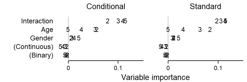
To understand why an interaction predictor “soaks up” predictive utility even though the data do not include an interaction, consider the situation where the interaction predictor is sampled alongside an unrelated variable (for instance, either the binary or the continuous noise variable). The splitting scheme then treats the interaction variable as a categorical predictor with four distinct levels. Due to the main effects that are present in the data, there are systematic differences among these subgroups. As a result, the algorithm will find a predictively useful split. This split will likely partition the data along the predictor age or gender, as these are related to the response variable. The interaction predictor will receive “Predictive credit” for this split, even though it is the variable age or gender that should be credited. As a result, the interaction predictor steals predictive power from each of these predictors. The variable importance scores we obtain are therefore not interpretable – they do not give accurate information and they do not tell us what we wanted to know. For amore in-depth discussion of this issue, please refer to Strobl et al. (2024).

Problem 2: Partial dependence plots of interaction variables do not provide a clean picture

To demonstrate the second issue, I will create data that do show a statistical interaction, both on the scale of outcome proportions and the logit scale. Then I will fit two RF models to these data, one without and one with an interaction predictor. I will then draw conditional partial dependence plots for both models.

Data

The data consist of 1,200 speakers, which are gain divided into four groups:

• 300 old, male
• 300 old, female
• 300 young, male
• 300 young, female

This means that there are again two binary predictors, gender (male vs. female) and age (young vs. old). For some binary outcome variable of interest, these are the percentages in the four cells:

• 20% old, male
• 30% old, female
• 45% young, male
• 80% young, female

Figure 3 shows the structure we have built into the data.

n_obs_per_cell <- 300

probs <- c(.2, .3, .45, .8)

condition_were <-probs * n_obs_per_cell


d <- data.frame(
  #speaker = paste0("subj_", 1:n_speakers),
  age = c("old", "old", "young", "young"),
  gender = c("male", "female", "male", "female"),
  were = condition_were,
  was = n_obs_per_cell - condition_were
) |> 
  pivot_longer(
    cols = c("was", "were"), 
    names_to = "variant", 
    values_to = "freq")

d <- expand.dft(d, freq = "freq") 

d$age <- factor(d$age)
d$gender <- factor(d$gender)
d$variant <- factor(d$variant)
d$interaction <- factor(d$age:d$gender)
d$random_continuous <- rnorm(nrow(d))
d$random_binary <- rbinom(nrow(d), 1, .5)

d <- d[order(d$variant, decreasing = TRUE),]

d |> group_by(age, gender) |> 
  dplyr::summarize(
    mean_prop = round(mean(variant == "were"), 2)
  ) |> ggplot(aes(x = age, y = mean_prop, group = gender)) +
  geom_point() +
  scale_y_continuous(
    limits = c(0,1), expand = c(0,0),
    breaks = c(0, .5, 1),
    labels = c("0", ".5", "1")) +
  geom_line() +
  annotate("text", x = 2.1, y = c(.45, .8) + .02, 
           label = c("male", "female"),
           size = 3.2, adj = 0) +
  ylab("Proportion of interest") +
  xlab(NULL) +
  theme_classic_ls()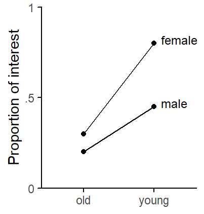

Figure 3: Line plot showing how the proportion of interest varies with age and gender.

We also add to the dataset two variables that represent random noise, a binary one (random_binary) and a continuous one (random_continuous).

Modeling

To examine the consequences of including the interaction predictor age:gender as an additional variable into the model, we will fit and compare two models, M1 and M2:

• M1 does not include an interaction predictor
  • formula: variant ~ age + gender + random_continuous + random_binary
• M2 includes an interaction predictor
  • formula: variant ~ age + gender + random_continuous + random_binary + interaction

For didactic purposes, we start by fitting a conditional inference tree to the full dataset using the function ctree() in the {party} package (Hothorn, Hornik, and Zeileis 2006). This conditional inference tree includes the manually specified predictor for the age-by-gender interaction. The resulting splitting scheme is shown in Figure 4. It includes three splits: two according to the interaction, and one according to gender. Surprisingly, age doesn’t appear at all as a splitting variable, which should make us skeptical.

d_tree <- ctree(
  variant ~ age + gender + interaction +
    random_continuous + random_binary, 
  data = d)

plot(d_tree)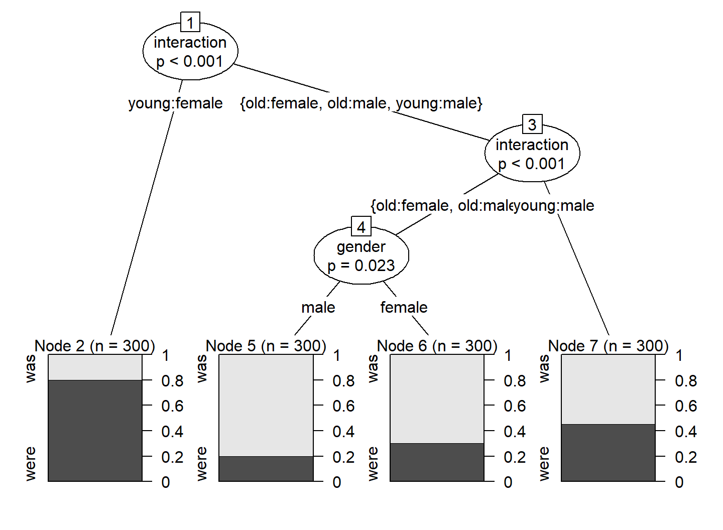

Figure 4: Conditional inference tree fit to the full dataset including an interaction predictor.

The next step is to fit two conditional random forest models (M1 and M2) using the function cforest() in the {party} package (Hothorn, Hornik, and Zeileis 2006).

rf_inter_1 <- party::cforest(
   variant ~ age + gender +
    random_continuous + random_binary, data = d,
      control = party::cforest_unbiased(
        mtry = 2, 
        ntree = 500))


rf_inter_2 <- party::cforest(
  variant ~ age + gender + interaction +
    random_continuous + random_binary, data = d,
      control = party::cforest_unbiased(
        mtry = 2, 
        ntree = 500))

Next, we compute conditional variable importance scores for each model, using the permimp package (Debeer, Hothorn, and Strobl 2025):

varimp_rf_inter_1 <- permimp::permimp(
  rf_inter_1,
  conditional = TRUE,
  progressBar = FALSE)$values


varimp_rf_inter_2 <- permimp::permimp(
  rf_inter_2,
  conditional = TRUE,
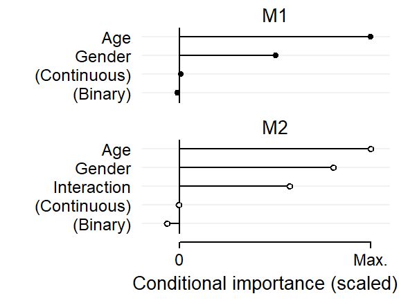
  progressBar = FALSE)$values

We start by inspecting the variable importance scores, which are shown in Figure 5. For comparison, I have scaled these in such a way that each plot extends to the maximum importance score in the respective model. This rescaling does not affect our interpretation here since the relevant benchmarks are the conditional importance scores for the predictors random_binary and random_continuous.

• For M1, the importance measures suggest that both age and gender have predictive utility, in line with the structure we have built into the data.
• For M2, it is age, gender and their interaction that emerge as predictively important, also in line with the structure we have built into the data.

xyplot(
  1~1, type = "n", xlim = c(-.2, 1.1), ylim = c(0, 12.5),
  par.settings = lattice_ls,
  xlab = "Conditional importance (scaled)",
  ylab = NULL,
  scales = list(
    x = list(at = c(0, 1), label = c("0", "Max.")),
    y = list(
      at = c(1:5, 8:11), label = c(
        "(Binary)", "(Continuous)", "Interaction", "Gender", "Age",
        "(Binary)", "(Continuous)", "Gender", "Age"
      )), cex = .9),
  panel = function(x,y){
    panel.segments(x0 = -.2, x1 = 1.1, y0 = c(1:5, 8:11), y1 = c(1:5, 8:11), 
                   col = "grey95")
    panel.segments(x0 = 0, x1 = 0, y0 = .5, y1 = 5.5)
    panel.segments(x0 = 0, x1 = 0, y0 = 7.5, y1 = 11.5)
    panel.segments(x0 = 0, x1 = sort(varimp_rf_inter_2$varimp_scaled),
                   y0 = 1:5, y1 = 1:5)
    panel.segments(x0 = 0, x1 = sort(varimp_rf_inter_1$varimp_scaled),
                   y0 = 8:11, y1 = 8:11)
    panel.points(x = sort(varimp_rf_inter_2$varimp_scaled), y = 1:5,
                 pch = 21, fill = "white", cex = 1.1)
    
    panel.points(x = sort(varimp_rf_inter_1$varimp_scaled), y = 8:11,
                 pch = 19, cex = 1)
    panel.segments(x0 = 0, x1 = 1, y0 = 0, y1 = 0)
    panel.segments(x0 = 0:1, x1 = 0:1, y0 = 0, y1 = -.3)
    panel.text(x = .5, y = c(6, 12)+.2, label = c("M2", "M1"), cex = 1)
  })

Figure 5: Conditional variable importance for the predictors in model with and without an interaction predictor.

Comparison of partial dependence scores

Finally, we obtain partial dependence scores based on each model. Since the main effects of age and gender as well as their interaction are the only patterns we have built into the data, a partial dependence plot for the predictor age conditional on gender should recover the pattern we saw in Figure 3. We use the partial() function in the pdp package (Greenwell 2017) to calculate the following partial dependence scores:

• M1: Partial dependence scores for age conditional on gender
• M2: Partial dependence scores for the interaction predictor
• M2: Partial dependence scores for age conditional on gender

pdp_1 <- pdp::partial(
  rf_inter_1, 
  pred.var = c("age", "gender"),
  type = "classification",
  #which.class = "were",
  prob = TRUE)

pdp_2 <- pdp::partial(
  rf_inter_2, 
  pred.var = "interaction",
  type = "classification",
  #which.class = "were",
  prob = TRUE)

pdp_2_maineffects <- pdp::partial(
  rf_inter_2, 
  pred.var = c("age", "gender"),
  type = "classification",
  #which.class = "were",
  prob = TRUE)

Figure 6 compares the results. Panel (a) at the far left shows, as a point of reference, descriptive statistics for the dataset. The plot is identical to Figure 3 above.

Panel (b) shows a conditional partial dependence plot for M1, the model without an interaction predictor. The partial dependence scores for age conditional on gender align very closely with the patterns we built into the data.

Panel (c) shows a partial dependence plot for the interaction predictor in M2. While the scores do give an idea of the interaction pattern, they also show traces of the two main effects: The scores for female speakers are higher, on average; and the scores for young speakers are also higher, on average.

Panel (d) shows partial dependence scores for age conditional on gender. The plot also shows a trace of the interaction between age and gender, indicating that the interaction effect is not entirely captured by the interaction predictor.

d_descr <- d |> group_by(age, gender) |> 
  dplyr::summarize(
    prop_were = mean(variant == "were")
  )

p0 <- xyplot(
  1 ~ 1, type = "n", ylim = c(0,1), xlim = c(.8, 2.2),
  par.settings = lattice_ls, axis = axis_L,
  xlab = NULL, ylab = "Proportion",
  scales = list(x = list(at = 1:2, labels = c("old", "young"), cex = .85),
                y = list(at = c(0, .5, 1), label = c("0", ".5", "1"))),
  xlab.top = list(label = "\n\n\nDescriptive\nstatistics\n", lineheight = .85, cex = .9),
  panel = function(x,y){
    panel.points(x = 1:2, y = d_descr$prop_were[c(1,3)], type="l")
    panel.points(x = 1:2, y = d_descr$prop_were[c(2,4)], type="l")
    panel.points(x = 1:2, y = d_descr$prop_were[c(1,3)], pch = 19, cex = 1)
    panel.points(x = 1:2, y = d_descr$prop_were[c(2,4)], pch = 21, fill = "white", cex = 1)
    panel.text(x = 1.5, y = .95, label = "(a)", col = "grey40")
  })


p1 <- xyplot(
  1 ~ 1, type = "n", ylim = c(0,1), xlim = c(.8, 2.2),
  par.settings = lattice_ls, axis = axis_L,
  xlab = NULL, ylab = NULL,
  scales = list(x = list(at = 1:2, labels = c("old", "young"), cex = .85),
                y = list(at = c(0, .5, 1), label = NULL)),
  xlab.top = list(label = "\n\n\nPDP\nInteraction\n", lineheight = .85, cex = .9),
  panel = function(x,y){
    panel.points(x = 1:2, y = 1-pdp_2$yhat[c(1,3)], type="l")
    panel.points(x = 1:2, y = 1-pdp_2$yhat[c(2,4)], type="l")
    panel.points(x = 1:2, y = 1-pdp_2$yhat[c(1,3)], pch = 19, cex = 1)
    panel.points(x = 1:2, y = 1-pdp_2$yhat[c(2,4)], pch = 21, fill = "white", cex = 1)
    panel.text(x = 2.45, y = 1.4, label = "\nModel including interaction", lineheight = .85, cex = .9)
    panel.segments(x0 = .8, x1 = 4.1, y0 = 1.27, y1  = 1.27)
    panel.text(x = 1.5, y = .95, label = "(c)", col = "grey40")
  })

p2 <- xyplot(
  1 ~ 1, type = "n", ylim = c(0,1), xlim = c(.8, 2.2),
  par.settings = lattice_ls, axis = axis_L,
  xlab = NULL, ylab = NULL,
  scales = list(x = list(at = 1:2, labels = c("old", "young"), cex = .85),
                y = list(at = c(0, .5, 1), label = NULL)),
  xlab.top = list(label = "\n\n\nConditional PDP\nAge, Gender\n", lineheight = .85, cex = .9),
  panel = function(x,y){
    panel.points(x = 1:2, y = 1-subset(pdp_2_maineffects, gender == "female",)$yhat, type="l")
    panel.points(x = 1:2, y = 1-subset(pdp_2_maineffects, gender == "male",)$yhat, type="l")
    panel.points(x = 1:2, y = 1-subset(pdp_2_maineffects, gender == "female",)$yhat, pch = 19, cex = 1)
    panel.points(x = 1:2, y = 1-subset(pdp_2_maineffects, gender == "male",)$yhat, pch = 21, fill = "white", cex = 1)
    panel.text(x = 1.5, y = .95, label = "(d)", col = "grey40")
    panel.text(x = 1.5, y = c(.25, .7), label = c("male", "female"), cex = .8)
  })

p3 <- xyplot(
  1 ~ 1, type = "n", ylim = c(0,1), xlim = c(.8, 2.2),
  par.settings = lattice_ls, axis = axis_L,
  xlab = NULL, ylab = NULL,
  scales = list(x = list(at = 1:2, labels = c("old", "young"), cex = .85),
                y = list(at = c(0, .5, 1), label = NULL)),
  xlab.top = list(label = "\n\n\nConditional PDP\nAge, Gender\n", lineheight = .85, cex = .9),
  panel = function(x,y){
    panel.points(x = 1:2, y = 1-subset(pdp_1, gender == "female",)$yhat, type="l")
    panel.points(x = 1:2, y = 1-subset(pdp_1, gender == "male",)$yhat, type="l")
    panel.points(x = 1:2, y = 1-subset(pdp_1, gender == "female",)$yhat, pch = 19, cex = 1)
    panel.points(x = 1:2, y = 1-subset(pdp_1, gender == "male",)$yhat, pch = 21, fill = "white", cex = 1)
    panel.text(x = 1.5, y = 1.4, label = "Model without\ninteraction", lineheight = .85, cex = .9)
    panel.text(x = 1.5, y = .95, label = "(b)", col = "grey40")
  })

cowplot::plot_grid(p0, NULL, p3, NULL, p1, NULL, p2, NULL, nrow = 1, rel_widths = c(1, -.1, 1, -.1, 1, -.1, 1, .1))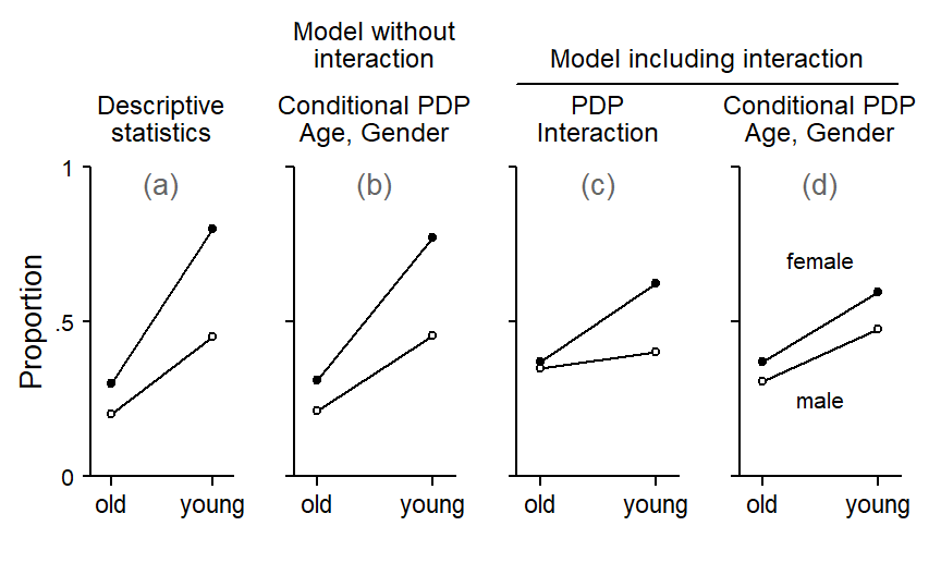

Figure 6: Partial dependence plots based on M1 (no interaction predictor) and M2 (with interaction predictor).

Figure 6 therefore shows that if the data include a pattern formed by both main and interaction effects, a model including a manually specified interaction predictor does not allow us to recover this pattern. At the same time, partial dependence scores do not allow us to isolate main-effect and interaction-effect components. Instead, the interaction predictor soaks up traces of the main effects of the constituent predictors and therefore yield a blended assessment.

In contrast, conditional partial dependence plots based on a model without manually specified interaction variables (panel b in Figure 6) provide a faithful representation of the patterns in the data.

Conclusion

It seems fair to say that the practice of including manually specified interaction variables should be discouraged in random-forest modeling. To detect relevant interactions in a random-forest model, researchers will need to stick to established methods such as Friedman’s H (Friedman and Popescu 2008), an index of interaction strength. To gauge the relative magnitude of interaction vs. main effects, (conditional) partial dependence plots need to be studied carefully.

References

Breiman, Leo. 1996. “Bagging Predictors.” Machine Learning 24 (2): 123–40. https://doi.org/10.1007/bf00058655.

Debeer, Dries, Torsten Hothorn, and Carolin Strobl. 2025. Permimp: Conditional Permutation Importance. https://doi.org/10.32614/CRAN.package.permimp.

Friedman, Jerome H., and Bogdan E. Popescu. 2008. “Predictive Learning via Rule Ensembles.” The Annals of Applied Statistics 2 (3). https://doi.org/10.1214/07-aoas148.

Greenwell, Brandon M. 2017. “Pdp: An R Package for Constructing Partial Dependence Plots.” The R Journal 9 (1): 421–36. https://doi.org/10.32614/RJ-2017-016.

Gries, Stefan Th. 2019. “On Classification Trees and Random Forests in Corpus Linguistics: Some Words of Caution and Suggestions for Improvement.” Corpus Linguistics and Linguistic Theory 16 (3): 617–47. https://doi.org/10.1515/cllt-2018-0078.

Hothorn, Torsten, Kurt Hornik, and Achim Zeileis. 2006. “Unbiased Recursive Partitioning: A Conditional Inference Framework.” Journal of Computational and Graphical Statistics 15 (3): 651–74. https://doi.org/10.1198/106186006X133933.

Sönning, Lukas. 2026. “Random Forests in Corpus Research: A Systematic Review.” January 13, 2026. https://osf.io/preprints/psyarxiv/byd5c_v1.

Strobl, Carolin, James Malley, and Gerhard Tutz. 2009. “An Introduction to Recursive Partitioning: Rationale, Application, and Characteristics of Classification and Regression Trees, Bagging, and Random Forests.” Psychological Methods 14 (4): 323–48. https://doi.org/10.1037/a0016973.

Strobl, Carolin, Yannick Rothacher, Sven Theiler, and Mirka Henninger. 2024. “Detecting Interactions with Random Forests: A Comment on Gries’ Words of Caution and Suggestions for Improvement.” Corpus Linguistics and Linguistic Theory, November. https://doi.org/10.1515/cllt-2024-0028.