Issues in random-forest modeling: Treatment of clustering variables

Corpus data often show a hierarchical structure, where observations are grouped by text/speaker or item. In this blog post, I comment on the practice of including clustering variables as predictors into a random-forest model. I demonstrate that this undermines the predictive utility of associated cluster-level predictors.

Author

Affiliation

Lukas Sönning

University of Bamberg

I recently did a systematic review on the use of random-forest models in corpus research (Sönning 2026). Perhaps unsurprisingly, 112 of the 125 RF models (90%) that entered this survey were fit to data with a grouping structure, where observations are clustered by text/speaker or item. In a considerable number of cases, the clustering variable was included into the RF model as an additional predictor variable:

• Of the 112 RF models with data clustered by speaker/text, 20 (18%) included the clustering variable into the analysis.
• Of the 80 RF models with data clustered by item (word form or lexeme), 5 (6%) included the clustering variable as a predictor.

In all cases, the clustering variable entered the analysis as an additional predictor, which means that the recursive partitioning scheme treated it on a par with the other variables in the model (i.e. as the equivalent of a fixed effect in a regression framework).

In this blog post, I want to comment on the situation where a clustering variable is included in an RF model alongside an associated cluster-level predictor. This is the case if a model includes, say, (i) the clustering variable speaker as well as speaker-level predictors such as age or gender; or (ii) the clustering variable word as well as word-level predictors such as frequency or word class.

In the survey I did, around half of the RF models that included a clustering variable also included a predictor that was measured at the cluster level:

• Of the 20 RFs including speaker as a predictor variable, 11 (55%) also had speaker/text-level predictors. Examples included: age, gender, education, generation, year of birth, ethnicity
• Of the 5 RFs that include item as a predictor variable, 3 (60%) also feature item-level predictors. Examples included: verb ending, verb modality, frequency, gradability, semantic category

I can see why some may think that including a clustering variable into an RF model might be a way of addressing the structure of the data – however, ordinary random forests do not handle clustering variables (e.g. speaker and item) appropriately. By “ordinary”, I mean RFs that do not take a mixed-effects approach to modeling clustering variables. In this blog post, I show that if these variables are included into a random-forest model, the “effect” of cluster-level predictors will be attenuated. Despite prominent precedent (Tagliamonte and Baayen 2012), then, this practice cannot be recommended. In this blog post, I use a simulated set of data to demonstrate this issue.

library(party)
library(permimp)
library(lattice)
library(vcdExtra)
library(tidyverse)
library(uls)

Simulate data

We start by simulating data with a binary response variable that is sensitive to speaker age and gender. The fictitious data include 50 speakers, with each individual contributing 30 observations to the data.

# set seed for reproducibility
set.seed(11)

# number of speaker and number of observations per speaker
n_speakers <- 50
n_tokens_per_speaker <- 30

# simulate speaker intercepts (on the logit scale)
speaker_intercepts_logit <- rnorm(n_speakers, 0, 1)

# simulate speaker age and gender
speaker_age <- (runif(n_speakers) -.5) * 4
speaker_gender <- rep(c(0,1), each = n_speakers/2)

# translate speaker intercepts to the proportion scale
speaker_intercepts_prob <- plogis(
  -speaker_age*.8 + (speaker_gender - .5) + speaker_intercepts_logit)

# use speaker-specific proportion to simulate binary outcome
speaker_were <- rbinom(
  n_speakers, n_tokens_per_speaker, speaker_intercepts_prob)

# obtain empirical proportion for each speaker
speaker_were_prop <- speaker_were/n_tokens_per_speaker


# organize these data into case form (one row per observation):
d <- data.frame(
  speaker = paste0("subj_", 1:n_speakers),
  age = speaker_age,
  gender = speaker_gender,
  were = speaker_were,
  was = n_tokens_per_speaker - speaker_were
) |> 
  pivot_longer(
    cols = c("was", "were"), 
    names_to = "variant", 
    values_to = "freq")

d <- expand.dft(d, freq = "freq") 

d$variant <- factor(d$variant)
d$speaker <- factor(d$speaker)
d$gender <- factor(d$gender, labels = c("male", "female"))

# add noise variables
d$random_continuous <- rnorm(nrow(d))
d$random_binary <- rbinom(nrow(d), 1, .5)

Figure 1 shows the patterns of association we have built into the data:

• The proportion of interest is linked to age: The younger the speaker, the lower the proportion.
• Speaker gender also plays a role, with male speakers showing a higher proportion.

p1 <- xyplot(
  speaker_were_prop ~ speaker_age, 
  groups = speaker_gender, pch = c(21,3), col = c("black", "black"), cex = c(1, .8),
  par.settings = lattice_ls, axis = axis_L, ylim = c(0,1),
  xlab = "Age", ylab = "Proportion of interest",
  scales = list(
    x = list(at = -1.5:1.5, label = rev(c(20, 40, 60, 80)), cex = .9),
    y = list(at = c(0, .5, 1), label = c("0", ".5", "1")), cex = .9),
  panel = function(x,y){
    #panel.abline(h = 0, col = "black")
    panel.points(x[speaker_gender == 0], y[speaker_gender == 0], lwd = .75, pch = 3, cex = .9, col = "black")
    panel.points(x[speaker_gender == 1], y[speaker_gender == 1], lwd = .75, pch = 21, cex = 1.1)
    
    panel.dotdiagram(speaker_were_prop[speaker_gender == 1], 
                     x_anchor = 2.6, seq_min = 0, seq_max = 1, 
                     n_bins = n_tokens_per_speaker, scale_y = .1, vertical = TRUE,
                     set_pch = 21, set_lwd = .75, set_cex = 1.1)
    
    panel.dotdiagram(speaker_were_prop[speaker_gender == 0], 
                     x_anchor = 3.6, seq_min = 0, seq_max = 1, 
                     n_bins = n_tokens_per_speaker, scale_y = .1, vertical = TRUE,
                     set_pch = 3, set_lwd = .75, set_cex = .9, set_col = "black")
    panel.text(x = c(2.6, 3.6), y = -.075, label = c("Male", "Female"), adj = 0, cex = 1, col = c("black", "black"))
  })

print(p1, position=c(0,0,.7,1))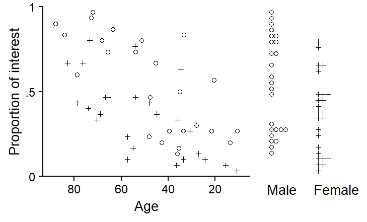

Figure 1: Scatterplot showing how the proportion of interest varies with age and gender.

We also add to the dataset two variables that represent random noise, a binary one (random_binary) and a continuous one (random_continuous). This is for two reasons:

• First, it will increase the number of predictors, making RF modeling (which includes predictor sampling) feasible
• Second, and more importantly, the variable importance scores we obtain for these noise variables are a useful point of reference for the predictors of interest. Due to the associations we have built into the model, age and gender should exceed both noise variables in predictive utility.

This is the resulting dataset:

str(d)

tibble [1,500 × 6] (S3: tbl_df/tbl/data.frame)
 $ speaker          : Factor w/ 50 levels "subj_1","subj_10",..: 1 1 1 1 1 1 1 1 1 1 ...
 $ age              : num [1:1500] 1.14 1.14 1.14 1.14 1.14 ...
 $ gender           : Factor w/ 2 levels "male","female": 1 1 1 1 1 1 1 1 1 1 ...
 $ variant          : Factor w/ 2 levels "was","were": 1 1 1 1 1 1 1 1 1 1 ...
 $ random_continuous: num [1:1500] -0.442 0.244 0.597 -0.12 -2.07 ...
 $ random_binary    : int [1:1500] 0 0 0 0 1 1 0 0 1 0 ...

Modeling

In what follows, we will examine the consequences of including the clustering variable speaker as an additional variable into the model. We will therefore fit and compare two models, M1 and M2:

• M1 does not include the clustering variable speaker
  • formula: variant ~ age + gender + random_continuous + random_binary
• M2 includes the clustering variable speaker
  • formula: variant ~ age + gender + random_continuous + random_binary + speaker

For didactic purposes, we start by fitting a conditional inference tree to the full dataset using the function ctree() in the {party} package (Hothorn, Hornik, and Zeileis 2006). The resulting splitting scheme is shown in Figure 2. It includes three splits: three according to speaker, and one according to gender. Surprisingly, age doesn’t appear at all as a splitting variable, which should make us skeptical.

d_tree <- party::ctree(
  variant ~ age + gender +
    random_continuous + random_binary +
    speaker, 
  data = d)

plot(d_tree)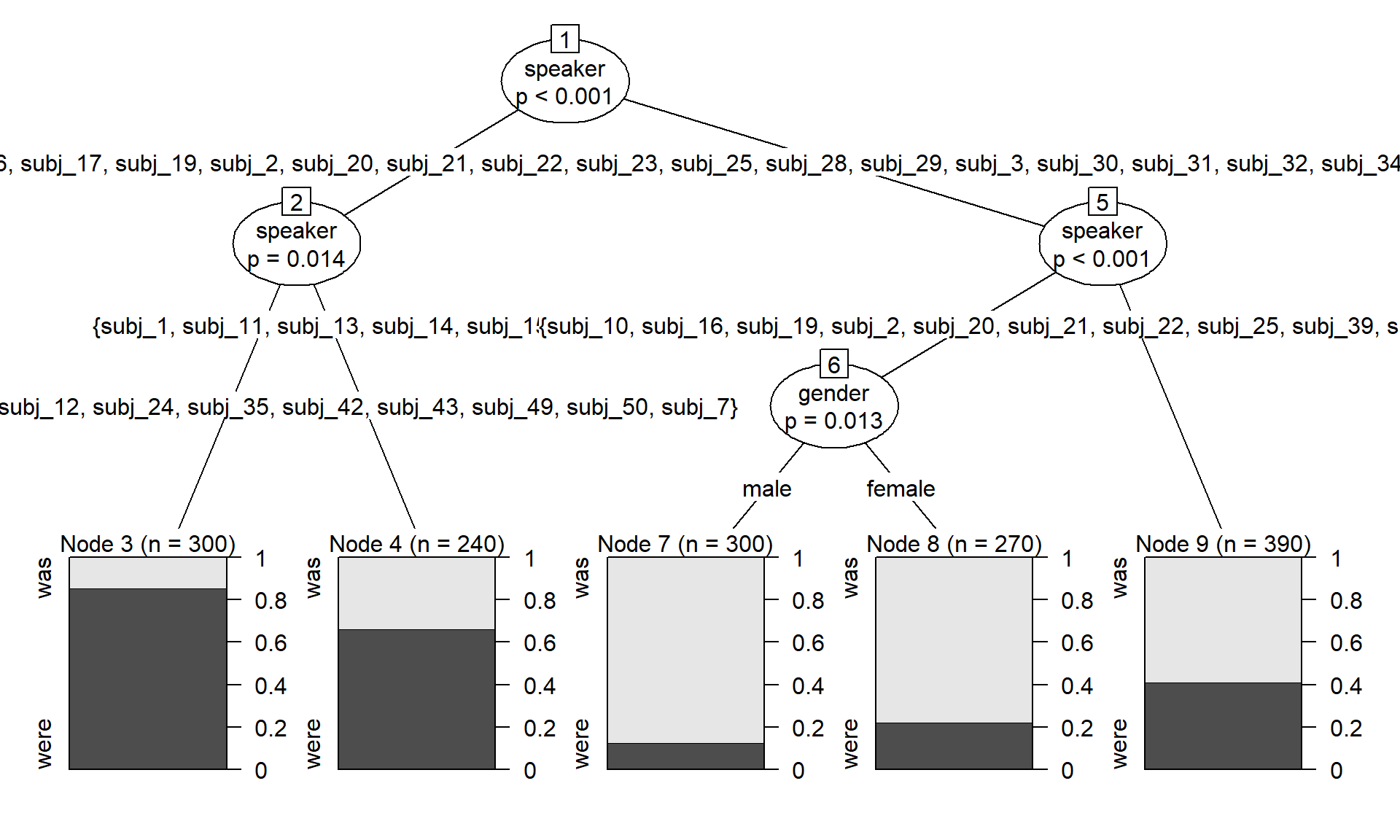

Figure 2: Conditional inference tree fit to the full dataset.

The next step is to fit two conditional random-forest models (M1 and M2) using the function cforest() in the {party} package (Hothorn, Hornik, and Zeileis 2006).

# M1
d_rf_1 <- party::cforest(
  variant ~ age + gender + 
    random_continuous + random_binary, 
  data = d,
  control = party::cforest_unbiased(
    mtry = 2, 
    ntree = 500))

# M2
d_rf_2 <- party::cforest(
  variant ~ 
    age + gender +
    random_continuous + random_binary + 
    speaker,  
  data = d,
  control = party::cforest_unbiased(
    mtry = 2, 
    ntree = 500))

Next, we compute conditional variable importance scores for each model, using the permimp package (Debeer, Hothorn, and Strobl 2025):

# M1
varimp_d_rf_1 <- permimp::permimp(
  d_rf_1,
  conditional = TRUE,
  progressBar = FALSE)$values

varimp_d_rf_1 <- as.data.frame(varimp_d_rf_1)
varimp_d_rf_1$variable <- rownames(varimp_d_rf_1)


# M2
varimp_d_rf_2 <- permimp::permimp(
  d_rf_2,
  conditional = TRUE,
  progressBar = FALSE)$values

varimp_d_rf_2 <- as.data.frame(varimp_d_rf_2)
varimp_d_rf_2$variable <- rownames(varimp_d_rf_2)

Finally, we obtain partial dependence scores for the predictors ageand gender for each model, using the partial() function in the pdp package (Greenwell 2017):

# M1
pdp_gender_1 <- pdp::partial(
  d_rf_1, 
  pred.var = "gender",
  type = "classification",
  which.class = "variant.were",
  prob = TRUE)

pdp_age_1 <- pdp::partial(
  d_rf_1, 
  pred.var = "age", 
  pred.grid = data.frame(
    age = seq(-2, 2, .25)),
  type = "classification",
  which.class = "variant.were",
  prob = TRUE)


# M2
pdp_gender_2 <- pdp::partial(
  d_rf_2, 
  pred.var = "gender",
  type = "classification",
  which.class = "variant.were",
  prob = TRUE)

pdp_age_2 <- pdp::partial(
  d_rf_2, 
  pred.var = "age", 
  pred.grid = data.frame(
    age = seq(-2, 2, .25)),
  grid.resolution = 10,  
  type = "classification",
  which.class = "variant.were",
  prob = TRUE)

Variable importance scores

We start by inspecting the variable importance scores, which are shown in the Figure 3. For comparison, I have scaled these in such a way that each plot extends to the maximum importance score in the respective model. This rescaling does not affect our interpretation here since the relevant benchmarks are the conditional importance scores for the predictors random_binary and random_continuous.

• For M1, the importance measures suggest that both age and gender have predictive utility, in line with the structure we have built into the data.
• For M2, it is age and speaker that emerge as predictively important; gender, however, ranks with the noise variables.

xyplot(
  1~1, type = "n", xlim = c(-.2, 1.1), ylim = c(0, 12.5),
  par.settings = lattice_ls,
  xlab = "Conditional importance (scaled)",
  ylab = NULL,
  scales = list(
    x = list(at = c(0, 1), label = c("0", "Max."), cex = .9),
    y = list(
      at = c(1:5, 8:11), label = c(
        "(Continuous)", "(Binary)", "Gender", "Speaker", "Age",
        "(Continuous)", "(Binary)", "Gender", "Age"
      )), cex = .9),
  panel = function(x,y){
    panel.segments(x0 = -.2, x1 = 1.1, y0 = c(1:5, 8:11), y1 = c(1:5, 8:11), 
                   col = "grey95")
    panel.segments(x0 = 0, x1 = 0, y0 = .5, y1 = 5.5)
    panel.segments(x0 = 0, x1 = 0, y0 = 7.5, y1 = 11.5)
    panel.segments(x0 = 0, x1 = sort(varimp_d_rf_2$varimp_scaled),
                   y0 = 1:5, y1 = 1:5)
    panel.segments(x0 = 0, x1 = sort(varimp_d_rf_1$varimp_scaled),
                   y0 = 8:11, y1 = 8:11)
    panel.points(x = sort(varimp_d_rf_2$varimp_scaled), y = 1:5,
                 pch = 21, fill = "white", cex = 1)
    
    panel.points(x = sort(varimp_d_rf_1$varimp_scaled), y = 8:11,
                 pch = 19, cex = 1)
    panel.segments(x0 = 0, x1 = 1, y0 = 0, y1 = 0)
    panel.segments(x0 = 0:1, x1 = 0:1, y0 = 0, y1 = -.3)
    panel.text(x = .5, y = c(6, 12)+.2, label = c("M2", "M1"), cex = 1)
  })

Figure 3: Conditional variable importance for the predictors in models M1 and M2.

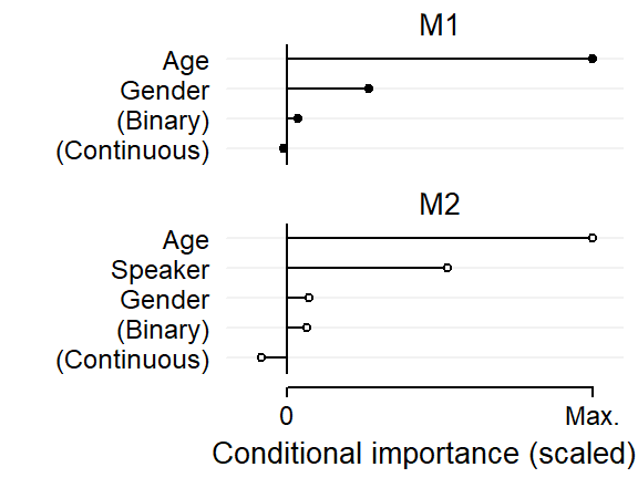
Apparently, the inclusion of the variable speaker has affected the predictive utility of the variable gender.

Partial dependence plots

To shed further light on this, we inspect partial dependence plots for the predictors age and gender based on both models. These are compared in Figure 4. It is clear from this figure that the inclusion of the clustering variable speaker has undermined the predictive power of both speaker-level variables: The partial dependence scores based on M1, which appear as open circles, are more extreme, indicating greater predictive discrimination for young vs. old and male vs. female individuals In contrast, partial dependence scores based on M2, which includes speaker, are flatter.

p1 <- xyplot(
  1~1, type = "n", xlim = c(-2.2, 2.2), ylim = c(0,1),
  par.settings = lattice_ls, axis = axis_L,
  xlab = "", ylab = "Proportion of interest",
  scales = list(
    x = list(at = -1.5:1.5, label = rev(c(20, 40, 60, 80)), cex = .9),
    y = list(at = c(0, .5, 1), label = c("0", ".5", "1")), cex = .9),
  panel = function(x,y){
    panel.points(x = pdp_age_2$age,
                 y = pdp_age_2$yhat, type = "l")
    
    panel.points(x = pdp_age_1$age,
                 y = pdp_age_1$yhat, type = "l")
    
    panel.points(x = pdp_age_2$age,
                 y = pdp_age_2$yhat, pch = 19, cex = 1.1)
    
    panel.points(x = pdp_age_1$age,
                 y = pdp_age_1$yhat, pch = 21, fill = "white", cex = 1.1)
    panel.text(x = 1.5, y = 1-c(.55, .9), 
               label = c("M2", "M1"), cex = .9)
    panel.text(x = -2.1, y = 1.07, label = " Age", adj = 0)
    panel.text(x = c(-2.1, -9.45), y = 1.15, label = c(
      " Partial dependence plots\n", "Conditional variable\nimportance scores (rescaled)"), adj = 0, lineheight = .85)
  })

p2 <- xyplot(
  1~1, type = "n", xlim = c(2.2, .8), ylim = c(0,1),
  par.settings = lattice_ls, axis = axis_L,
  xlab = "", ylab = " ",
  scales = list(
    x = list(at = 1:2, label = c("Male", "Female"), cex = .9),
    y = list(at = c(0, .5, 1), label = c("0", ".5", "1")), cex = .9),
  panel = function(x,y){
    panel.points(x = pdp_gender_2$gender,
                 y = pdp_gender_2$yhat, type = "l")
    
    panel.points(x = pdp_gender_1$gender,
                 y = pdp_gender_1$yhat, type = "l")
    
    panel.points(x = pdp_gender_2$gender,
                 y = pdp_gender_2$yhat, pch = 19, cex = 1.1)
    
    panel.points(x = pdp_gender_1$gender,
                 y = pdp_gender_1$yhat, pch = 21, fill = "white", cex = 1.1)
    panel.text(x = 1.9, y = 1-c(.33, .63), 
               label = c("M1", "M2"), cex = .9)
    panel.text(x = 2.2, y = 1.07, label = " Gender", adj = 0)
  })

print(p1, position = c(0,-.1,.65,.86), more = TRUE)
print(p2, position = c(.6,-.1, 1,.86))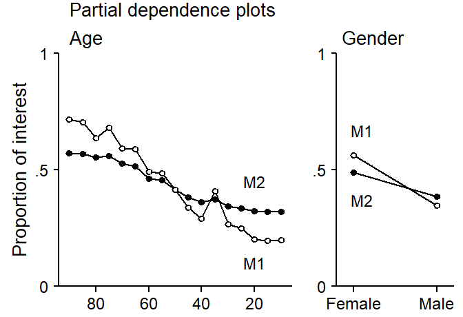

Figure 4: Partial dependence plots for age and gender in models M1 and M2.

We can compare the “steepness” of the profiles numerically, by looking at the range of the partial dependence scores for the two models:

• age
  • M1: .52 (Min: .20; Max: .72)
  • M2: .25 (Min: .32; Max: .57)
• gender
  • M1: .22 (Min: .35; Max: .56)
  • M2: .10 (Min: .39; Max: .49)

Understanding why

To understand why the inclusion of clustering variables undermines the predictive utility of the associated cluster-level predictors, it is instructive to inspect the first split in the conditional inference tree shown in Figure 2. The first split is made on speaker, and 18 individuals are assigned to the left branch, 32 to the right branch. The sample is therefore divided into two groups. The scatterplot in Figure 5 shows that this split is made at a proportion of around .55. The subset of speakers in the left branch is colored in gray, the ones in the right branch in blue.

For this split, the prediction scheme assigns predictive value to the variable speaker only. This is despite the fact that the two subgroups differ systematically with regard to the distribution of age and gender. This is clarified in the plots added at the top of Figure 5:

• The bar chart shows that the right branch (blue) includes a greater proportion of male speakers (63% vs. 28% in the right branch). Recall that male speakers were simulated to have lower proportions (see Figure 1).
• The boxplot shows that the right branch (blue) also includes speakers who are, on average, younger (median age 33 vs. 62 years). Recall that younger speakers were simulated to have lower proportions (see Figure 1).

# speaker summary
d_summary <- d |> group_by(speaker) |> 
  dplyr::summarize(
    age = unique(age),
    gender = unique(gender),
    prop_were = mean(variant == "were")
  )

d_tree <- ctree(
  variant ~ age + gender + speaker +
    random_continuous + random_binary, 
  data = d)

speaker_split <- d_tree@tree$psplit$splitpoint

speakers_to_the_left <- levels(speaker_split)[as.logical(speaker_split)]
speakers_to_the_right <- levels(speaker_split)[as.logical(speaker_split*-1+1)]

d_summary$branch <- factor(
  c("right", "left")[as.numeric(d_summary$speaker %in% speakers_to_the_left)+1])


# draw plot
p1 <- xyplot(
  prop_were ~ age, 
  col = col_ls[c(1,3)][as.numeric(d_summary$branch)], 
  pch = c(3,1)[as.numeric(d_summary$gender)],
  cex = 1,
  data = d_summary,
  xlab = "Age", ylab = "Proportion of interest", ylim = c(0,1),
  par.settings = lattice_ls, axis = axis_L,
scales = list(
    x = list(at = -1.5:1.5, label = rev(c(20, 40, 60, 80))),
    y = list(at = c(0, .5, 1), label = c("0", ".5", "1"))),
panel = function(x,y,...){
  panel.xyplot(x,y,...)
  panel.segments(x0 = 2.5, x1 = 2.5, col = col_ls[1],
                 y0 = min(y[d_summary$branch == "left"]),
                 y1 = max(y[d_summary$branch == "left"]))
  panel.segments(x0 = 2.4, x1 = 2.5, col = col_ls[1],
                 y0 = range(y[d_summary$branch == "left"]),
                 y1 = range(y[d_summary$branch == "left"]))
  
  panel.segments(x0 = 2.5, x1 = 2.5,col = col_ls[3],
                 y0 = min(y[d_summary$branch == "right"]),
                 y1 = max(y[d_summary$branch == "right"]))
  panel.segments(x0 = 2.4, x1 = 2.5,col = col_ls[3],
                 y0 = range(y[d_summary$branch == "right"]),
                 y1 = range(y[d_summary$branch == "right"]))
  
  panel.text(x = 2.7, y = c(.25, .75), label = c(
    "Assigned to\nright branch\n(n = 32)", "Assigned to\nleft branch\n(n = 18)"
  ), lineheight = .85, adj = 0, cex = .9, col = col_ls[c(3,1)])
    })

p2 <- bwplot(reorder(branch, -age) ~ age, data = d_summary,
  par.settings = lattice_ls, box.ratio = 4,
  scales = list(x = list(draw = FALSE),
                y = list(cex = .9)),
  fill = fill_ls[c(3,1)],
  xlab = NULL,
  panel = function(x,y,...){
    panel.bwplot(x,y,...)   
    panel.text(x = 2.7, y = 3, label = "Median age", cex = .9, adj = 0)
    panel.text(x = 2.7, y = 2, label = "  Left branch: 33 years", cex = .9, adj = 0, col = col_ls[1])
    panel.text(x = 2.7, y = 1, label = "  Right branch: 62 years", cex = .9, adj = 0, col = col_ls[3])
  })

d_barchart <- data.frame(
  prop.table(
    table(d_summary$gender, d_summary$branch), margin = 2))


p3 <- barchart(
  reorder(Var2, -as.numeric(Var2)) ~ Freq, groups = Var1:Var2,
               data = d_barchart, stack = TRUE,
  par.settings = lattice_ls, box.ratio = 4,
  xlab = NULL,
  scales = list(x = list(draw = FALSE),
                y = list(cex = .9)),
  col = c(
    fill_ls[1],
    fill_ls[3], 
    "white",
    "white"),
  panel = function(x,y,...){
    panel.barchart(x,y,...)
    panel.text(x = c(.1, .88), y = 2.95, label = c("male", "female"), cex = .9)
    panel.text(x = 1.19, y = 3, label = "Proportion male", cex = .9, adj = 0)
    panel.text(x = 1.19, y = 2, label = "  Left branch: 28%", cex = .9, adj = 0, col = col_ls[1])
    panel.text(x = 1.19, y = 1, label = "  Right branch: 63%", cex = .9, adj = 0, col = col_ls[3])
  })

print(p1, position = c(0,0,.62,.6), more = TRUE)
print(p2, position = c(-.02,.625,.625,.8), more = TRUE)
print(p3, position = c(-.02,.8,.625,.975))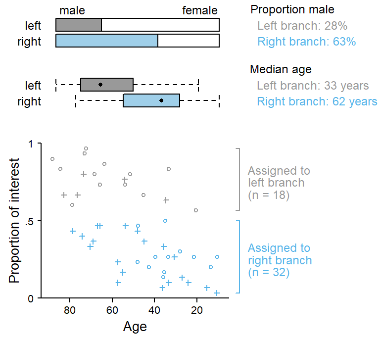

Figure 5: Explanation of the decrease in predictive utility of cluster-level variables in M2.

Since we have built the data, we know that part of the difference between the two subgroups of speakers (grey and blue) is systematic, i.e. attributable to age and gender. For this particular split, however, the tree records no information about systematic differences between grey and blue individuals. Instead, predictive credit is given exclusively to speaker. Since the right branch (blue) mostly includes younger speakers, predictive power has been robbed from age and instead assigned to speaker. And the same is true for gender: Since the right branch (blue) mostly includes male speakers, predictive power has also been robbed from gender and instead assigned to speaker.

Conclusion

Corpus data are often structured hierarchically, which poses a problem for random-forest modeling. We know from the regression context that ignoring clustering variables during data analysis is likely to yield overoptimistic models. Including clustering variables into an ordinary random-forest model has its own problems, however, one of which was discussed in the current blog post. If the data are to be analyzed with a random-forest model, the only way out of this dilemma is offered by mixed-effects random forests. For categorical response variables (i.e. classification tasks), such methods have emerged only recently (Pellagatti et al. 2021). If you come across an implementation of these models in R (or Python), spread the word!

References

Debeer, Dries, Torsten Hothorn, and Carolin Strobl. 2025. Permimp: Conditional Permutation Importance. https://doi.org/10.32614/CRAN.package.permimp.

Greenwell, Brandon M. 2017. “Pdp: An R Package for Constructing Partial Dependence Plots.” The R Journal 9 (1): 421–36. https://doi.org/10.32614/RJ-2017-016.

Hothorn, Torsten, Kurt Hornik, and Achim Zeileis. 2006. “Unbiased Recursive Partitioning: A Conditional Inference Framework.” Journal of Computational and Graphical Statistics 15 (3): 651–74. https://doi.org/10.1198/106186006X133933.

Pellagatti, Massimo, Chiara Masci, Francesca Ieva, and Anna M. Paganoni. 2021. “Generalized Mixed‐effects Random Forest: A Flexible Approach to Predict University Student Dropout.” Statistical Analysis and Data Mining: The ASA Data Science Journal 14 (3): 241–57. https://doi.org/10.1002/sam.11505.

Sönning, Lukas. 2026. “Random Forests in Corpus Research: A Systematic Review.” January 13, 2026. https://osf.io/preprints/psyarxiv/byd5c_v1.

Tagliamonte, Sali A., and R. Harald Baayen. 2012. “Models, Forests, and Trees of York English:was/Werevariation as a Case Study for Statistical Practice.” Language Variation and Change 24 (2): 135–78. https://doi.org/10.1017/s0954394512000129.