Drawing spike graphs to examine dispersion across text files

corpus linguistics
dispersion
data visualization
This blog post describes how to draw spike graphs that visualize the dispersion of an item across the text files in a corpus. These graphs are enriched with information about corpus design (and structure).
Author
Affiliation

University of Bamberg

Published

November 12, 2025

R setup
# install development version directly from Github
#pak::pak("lsoenning/tlda")
#pak::pak("lsoenning/wls")

library(tlda)      # for access to datasets
library(wls)       # for custom ggplot theme
library(tidyverse) # for data wrangling
library(ggh4x)     # for drawing nested facets in ggplot

source("C:/Users/ba4rh5/Work Folders/My Files/R projects/my_utils_website.R")

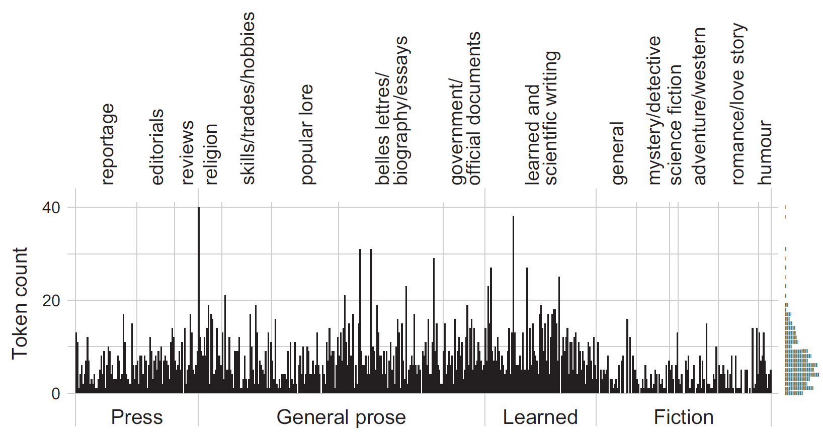
I first came across spike graphs as a tool for visualizing the dispersion of an item in a corpus in a paper by Church and Gale (1995). Since this graph type is a great visual aid for examining and illustrating the distribution of an item across the text files in a corpus, I have since started to use spike graphs in my own work (e.g. Figure 8 in Sönning -Sönning (2025a) and Figure 2 in Sönning -Sönning (2025b)). The following figure, which appears in Sönning (2025a, 21), shows the distribution of which across the 500 text files in the Brown Corpus. Each spike denotes a text file, and gaps represent documents that contain no instances of this item. Text files are grouped by macro genre (four categories marked at the bottom), and genre (15 categories marked at the top). The ‘hairy’ appearance of the spike graph indicates that which is a common word – it appears in almost every document. In this blog post, I describe how to draw such annotated spike graphs in R using the {ggplot2} package.

Spike graph showing the distribution of which in the Brown Corpus

Data format

To draw a spike graph, we need the following data for each text file in the corpus:

  • The frequency of the item in the text file
  • The length of the text file (number of word (and non-word) tokens)
  • Text metadata (e.g. mode, macro genre, genre, subgenre)

Our illustrative item will be actually, and we will look at its distribution in ICE-GB (Nelson, Wallis, and Aarts 2002). Frequency information for actually in the 500 text files in ICE-GB is available in the dataset biber150_ice_gb (see help("biber150_ice_gb")), which is part of the {tlda} package (Sönning 2025c). Let’s look at a small excerpt from this object, which is a term-document matrix:

  • Each column represents a text file
  • Each row represents an item (except for row 1, word_count, which gives the length of the text file)
biber150_ice_gb[1:10, 1:8]
           s1a-001 s1a-002 s1a-003 s1a-004 s1a-005 s1a-006 s1a-007 s1a-008
word_count    2195    2159    2287    2290    2120    2060    2025    2177
a               50      38      44      67      35      34      37      29
able             2       4       4       0       0       0       0       0
actually         3       6       2       2       6       3       0       8
after            0       0       0       0       4       1       1       0
against          0       0       0       0       0       0       0       0
ah               1       0       0       0       1       6       1       2
aha              0       0       0       0       0       0       0       0
all              2       5       6       9       7       5       8      13
among            0       0       0       0       0       0       0       0

We extract the relevant data for actually. Importantly, this table includes every text file in the corpus, even if the number of occurrences of actually is 0.

ice_actually <- data.frame(
  text_file = colnames(biber150_ice_gb),
    n_tokens = biber150_ice_gb[4,],
    word_count = biber150_ice_gb[1,]
)

str(ice_actually)
'data.frame':   500 obs. of  3 variables:
 $ text_file : chr  "s1a-001" "s1a-002" "s1a-003" "s1a-004" ...
 $ n_tokens  : num  3 6 2 2 6 3 0 8 2 6 ...
 $ word_count: num  2195 2159 2287 2290 2120 ...

Now we need to add metadata for the 500 text files, which are provided in the dataset metadata_ice_gb in the {tlda} package (Sönning 2025c). See help("metadata_ice_gb") for more information about this data table.

str(metadata_ice_gb)
'data.frame':   500 obs. of  7 variables:
 $ text_file    : chr  "s1a-001" "s1a-002" "s1a-003" "s1a-004" ...
 $ mode         : chr  "spoken" "spoken" "spoken" "spoken" ...
 $ text_category: Ord.factor w/ 4 levels "dialogues"<"monologues"<..: 1 1 1 1 1 1 1 1 1 1 ...
 $ macro_genre  : Ord.factor w/ 12 levels "private_dialogues"<..: 1 1 1 1 1 1 1 1 1 1 ...
 $ genre        : Ord.factor w/ 32 levels "face_to_face_conversations"<..: 1 1 1 1 1 1 1 1 1 1 ...
 $ genre_short  : Ord.factor w/ 32 levels "con"<"ph"<"les"<..: 1 1 1 1 1 1 1 1 1 1 ...
 $ word_count   : int  2195 2159 2287 2290 2120 2060 2025 2177 2063 2146 ...

Importantly, the classification variables denoting text varieties (text_category, macro_genre, and genre) are already ordered based on the sampling frame that informs the design of the ICE family of corpora. In metadata_ice_gb, they are represented as ordered factors. This is important for visualization, because we want to order the text files (and higher-level text categories) in a sensible way.

Next, we combine the two tables. The linking column is text_file, which allows us to join ice_gb with metadata_ice_gb:

ice_actually <- full_join(
  ice_actually, 
  metadata_ice_gb)

This yields a data frame with more information about each token in the corpus:

str(ice_actually)
'data.frame':   500 obs. of  8 variables:
 $ text_file    : chr  "s1a-001" "s1a-002" "s1a-003" "s1a-004" ...
 $ n_tokens     : num  3 6 2 2 6 3 0 8 2 6 ...
 $ word_count   : num  2195 2159 2287 2290 2120 ...
 $ mode         : chr  "spoken" "spoken" "spoken" "spoken" ...
 $ text_category: Ord.factor w/ 4 levels "dialogues"<"monologues"<..: 1 1 1 1 1 1 1 1 1 1 ...
 $ macro_genre  : Ord.factor w/ 12 levels "private_dialogues"<..: 1 1 1 1 1 1 1 1 1 1 ...
 $ genre        : Ord.factor w/ 32 levels "face_to_face_conversations"<..: 1 1 1 1 1 1 1 1 1 1 ...
 $ genre_short  : Ord.factor w/ 32 levels "con"<"ph"<"les"<..: 1 1 1 1 1 1 1 1 1 1 ...

And finally, to have nicer labels in the plot, I will replace the “_” symbols in the macro genre labels with an empty space. This is optional.

ice_actually$macro_genre_nice <- factor(
    ice_actually$macro_genre,
    labels = str_replace(
      levels(ice_actually$macro_genre), 
      pattern = "_",
      replacement = " "))

saveRDS(ice_actually, "ice_actually.rds")

Drawing the spike graph

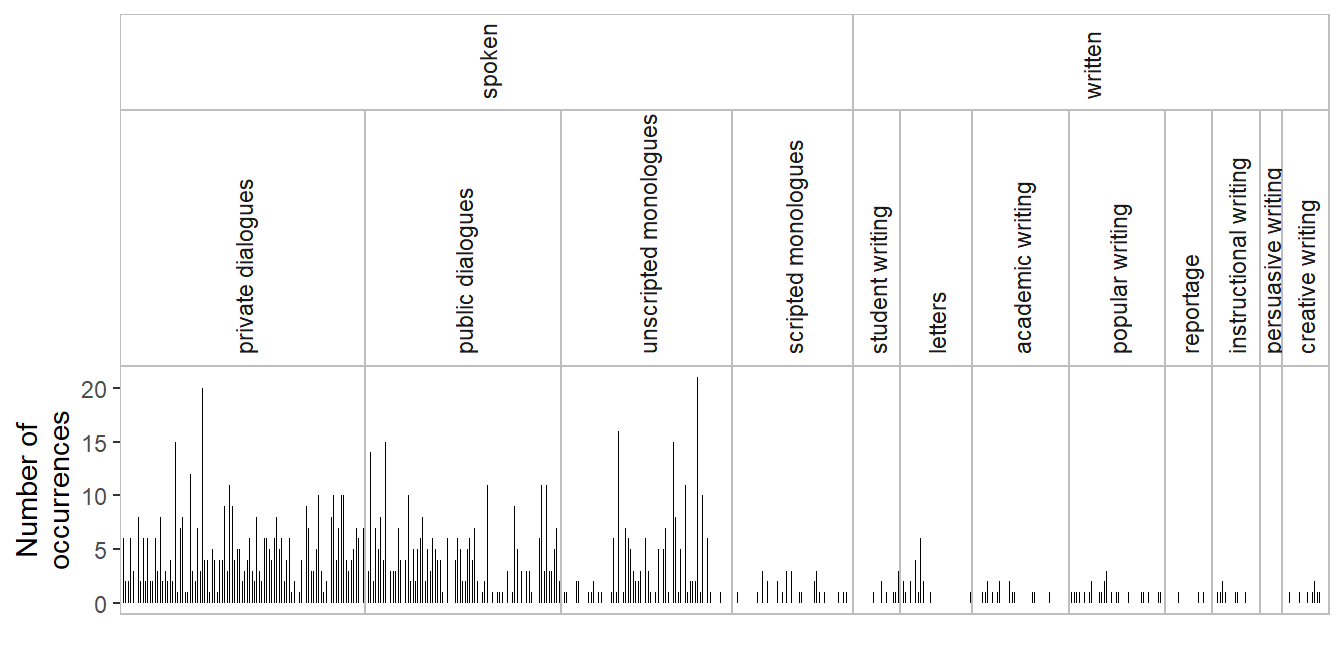
Now we are ready for plotting. The following annotated code draws a spike graph. It uses the function facet_nested() from the {ggh4x} package (van den Brand 2024) to draw nested facets. The function theme_spike_graph() from the {wls} package (Sönning 2025d) adjusts the ggplot2 theme for a clean appearance. In the following figure, we add two structural annotation layers as facets above the graph: mode (2 categories) and macro genre (12 categories):

ice_actually |> 
  ggplot(aes(x = text_file,            # text_file as x-variable
             y = n_tokens)) +          # frequency of item as y-variable
  geom_segment(aes(xend = text_file),  # draw spikes for each text file
               yend = 0,               #   spike starts at 0
               linewidth = .2) +       #   draw thin lines
  facet_nested(                        # nested facets with the {ggh4x} package:
    . ~ mode + macro_genre_nice,       #   macro genre facets nested within mode 
    scales = "free",                   #   allow x-scale to vary across facets
    space = "free_x",                  #   facet width proportional to # of texts
    strip = strip_nested(              #   allow height of facet labels above
      size = "variable")) +            #     graph to vary 
  theme_bw() +                         # specify theme_bw() as basis
  theme_spike_graph() +                # custom theme for spike graph
    scale_x_discrete(expand = c(0,0)) +  # avoid left/right padding in facets 
  ylab("Number of\noccurrences") +     # add y-axis title
  xlab("")  +                          # no title on x-axis
  theme(                               # 
    strip.text.x.top = element_text(   # format facet labels
      angle = 90, hjust = 0))          #   rotate by 90 degrees and left-align
Figure 1: Spike graph showing the distribution of actually in ICE-GB: Number of occurrences (absolute frequency) in each text file.

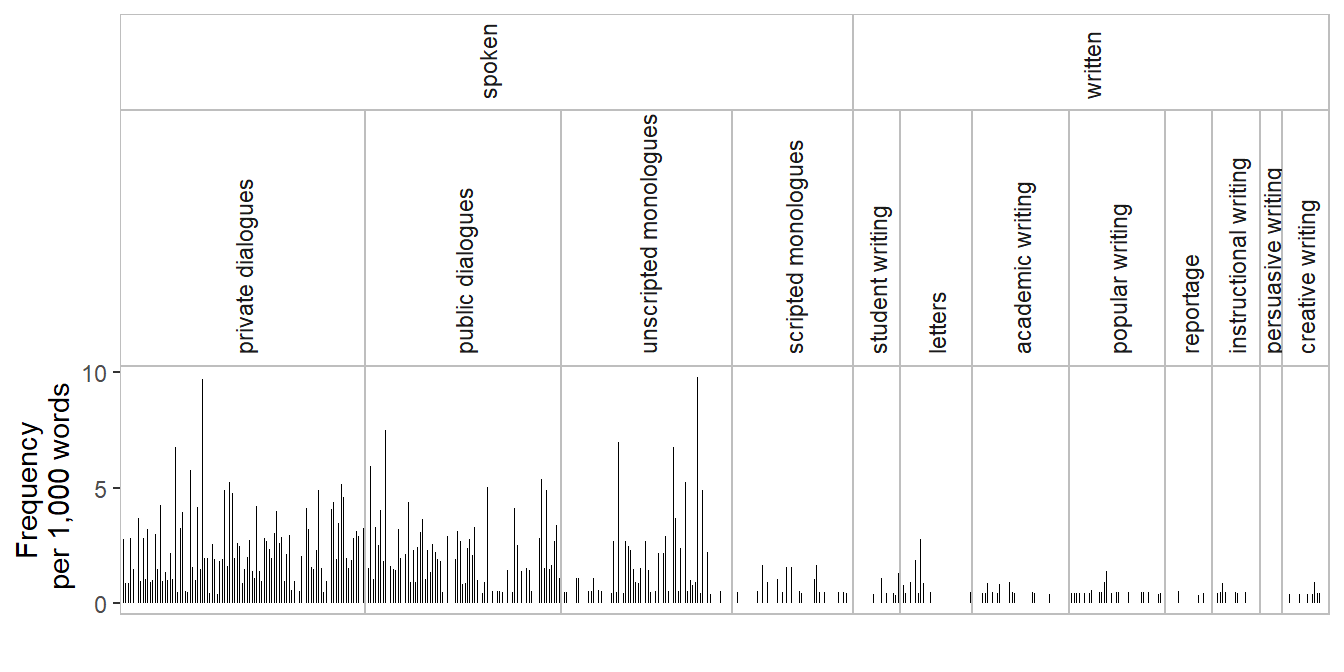
Spike graph showing normalized frequencies

Since the text files in ICE-GB are all around 2,000 words long, it was OK for our spike graph to show the number of occurrences of actually in each text file (i.e. absolute frequencies). It is usually more appropriate, however, to show relative frequencies (i.e. normalized frequencies), because text files will differ in length. Doing so requires an intermediate step: We add a column to the data frame ice_actually, which gives the normalized frequency of actually in the text file. Here, we opt for frequency per 1,000 words as a basis:

ice_actually$rate_ptw <- (ice_actually$n_tokens / ice_actually$word_count) * 1000
str(ice_actually)
'data.frame':   500 obs. of  10 variables:
 $ text_file       : chr  "s1a-001" "s1a-002" "s1a-003" "s1a-004" ...
 $ n_tokens        : num  3 6 2 2 6 3 0 8 2 6 ...
 $ word_count      : num  2195 2159 2287 2290 2120 ...
 $ mode            : chr  "spoken" "spoken" "spoken" "spoken" ...
 $ text_category   : Ord.factor w/ 4 levels "dialogues"<"monologues"<..: 1 1 1 1 1 1 1 1 1 1 ...
 $ macro_genre     : Ord.factor w/ 12 levels "private_dialogues"<..: 1 1 1 1 1 1 1 1 1 1 ...
 $ genre           : Ord.factor w/ 32 levels "face_to_face_conversations"<..: 1 1 1 1 1 1 1 1 1 1 ...
 $ genre_short     : Ord.factor w/ 32 levels "con"<"ph"<"les"<..: 1 1 1 1 1 1 1 1 1 1 ...
 $ macro_genre_nice: Ord.factor w/ 12 levels "private dialogues"<..: 1 1 1 1 1 1 1 1 1 1 ...
 $ rate_ptw        : num  1.367 2.779 0.875 0.873 2.83 ...

Then we can draw the plot. The annotations in the code below flag the changes we have made.

ice_actually |> 
  mutate(                                    # add column with normalized frequency
    rate_ptw = n_tokens / word_count * 1000  #   (per thousand words)
  ) |> 
  ggplot(aes(x = text_file,
             y = rate_ptw)) +                # normalized frequency as y-variable
  geom_segment(aes(xend = text_file),
               yend = 0,
               linewidth = .2) +
  facet_nested(
    . ~ mode + macro_genre_nice,
    scales = "free",
    space = "free_x",
    strip = strip_nested(
      size = "variable")) +
  theme_bw() +
  theme_spike_graph() +
    scale_x_discrete(expand = c(0,0)) +
  ylab("Frequency\n per 1,000 words") +      # change title of y-axis
  scale_y_continuous(breaks = c(0, 5, 10)) + # nicer tick marks on y-axis
  xlab("")  +
  theme(
    strip.text.x.top = element_text(
      angle = 90, hjust = 0))
Figure 2: Spike graph showing the distribution of actually in ICE-GB: Rate of occurrence (normalized frequency) in each text file.

References

Church, Kenneth W., and William A. Gale. 1995. “Poisson Mixtures.” Natural Language Engineering 1 (2): 163–90. https://doi.org/10.1017/s1351324900000139.
Nelson, Gerald, Sean Wallis, and Bas Aarts. 2002. Exploring Natural Language: Working with the British Component of the International Corpus of English. John Benjamins. https://doi.org/10.1075/veaw.g29.
Sönning, Lukas. 2025a. “Advancing Our Understanding of Dispersion Measures in Corpus Research.” Corpora 20 (1): 3–35. https://doi.org/10.3366/cor.2025.0326.
———. 2025b. “Dispersion Analysis.” OSF Preprints. https://doi.org/10.31219/osf.io/h3dyx_v2.
———. 2025c. Tlda: Tools for Language Data Analysis. https://github.com/lsoenning/tlda.
———. 2025d. Wls: R Utilities for Workshops Taught by Lukas Soenning. https://github.com/lsoenning/wls.
van den Brand, Teun. 2024. Ggh4x: Hacks for ’Ggplot2’. https://doi.org/10.32614/CRAN.package.ggh4x.

Citation

BibTeX citation:
@online{sönning2025,
  author = {Sönning, Lukas},
  title = {Drawing Spike Graphs to Examine Dispersion Across Text Files},
  date = {2025-11-12},
  url = {https://lsoenning.github.io/posts/2025-11-12_dispersion_spike_graph/},
  langid = {en}
}
For attribution, please cite this work as:
Sönning, Lukas. 2025. “Drawing Spike Graphs to Examine Dispersion Across Text Files.” November 12, 2025. https://lsoenning.github.io/posts/2025-11-12_dispersion_spike_graph/.