
R setup
library(tlda)
library(lattice)
library(knitr)
library(kableExtra)
library(uls) # pak::pak("lsoenning/uls")library(tlda)
library(lattice)
library(knitr)
library(kableExtra)
library(uls) # pak::pak("lsoenning/uls")In a recent paper, R. N. Nelson (2025) argues that corpus-based dispersion analysis should be informed by probabilistic models that take into account sampling variation (which he refers to as “noise”). This makes sense: Suppose we are interested in the dispersion of an item across (say) 10 registers, which are represented by sub-corpora. Even if the underlying usage rate (i.e. the true rate of occurrence of the item) is exactly the same in each register, the (normalized) frequencies observed in the sub-corpora will not be identical. This is due to sampling variation. Each sub-corpus is a sample from the target sub-population (i.e. register), and the sample statistic will fluctuate around the true value. The smaller the sample, the larger the fluctuation (i.e. sampling variation).
What R. N. Nelson (2025) finds problematic about existing parts-based measures is that they take an ideal, equally-apportioned distribution as a point of reference. Any deviation from this ideal moves the dispersion score away from the optimum. In my view, R. N. Nelson (2025) rightly argues that this benchmark is too strict and therefore unattainable. What is needed instead, he says, is a point of reference that provides some leeway in that it acknowledges the existence of sampling variation. This can be achieved with a probabilistic model such as the Poisson distribution, which is able to mark out the amount of sampling variation we must expect for a sample (i.e. corpus part) of a given size.
In fact, the Poisson distribution provides a probabilistic model for an item whose underlying (i.e. actual) usage rate in the population is constant across the contexts represented by corpus parts. If all parts are (say) 1,000 words long, and the underlying usage rate is 1 per thousand words, this model says how likely it is to observe a frequency count of 0, 1, 2, etc. The Poisson distribution therefore tells us how the subfrequencies will vary due to sampling variation, and this allows us to see how tolerant we should be to deviations from a perfectly even distribution.
This motivates R. N. Nelson (2025) to build a dispersion measure based on the Poisson model. The basic idea is straightforward. We first determine how many empty parts we would expect on the basis of the Poisson model. We express this as the expected Poisson-based probability of an empty part (i.e. a subfrequency of zero), \(\textrm{Pr}_{\textrm{exp}}(0)\). This provides the point of reference, which represents a scenario of perfect evenness, with a constant underlying usage rate throughout the target population. Then we compare the observed proportion of empty parts to this point of reference.
Suppose the Poisson distribution tells us that the probability of seeing a subfrequency of zero is .65. The expected proportion of empty corpus parts is therefore .65. If the observed proportion of empty corpus parts is near .65, the data are consistent with the Poisson model and therefore consistent with a maximally even/balanced distribution. If the observed proportion is higher, however, the data deviate from this ideal, resulting in the dispersion score moving away from the optimum.
To calculate MB, we therefore need to determine two quantities:
With these, we determine what R. N. Nelson (2025) calls biasedness, \(b\), which is the amount of deviation from evenness (i.e. from the Poisson model):
\[ b = \frac{|\textrm{Pr}_{\textrm{obs}}(0) - \textrm{Pr}_{\textrm{exp}}(0)|}{1 - \textrm{Pr}_{\textrm{exp}}(0)} \]
The value of MB is then equal to \(b\) unless the observed proportion of empty parts is smaller than (or equal to) the expected one:
\[ MB = \begin{cases} 0 & \textrm{if} & \textrm{Pr}_{\textrm{obs}}(0) \le \textrm{Pr}_{\textrm{exp}}(0)\\ b & \textrm{if} & \textrm{Pr}_{\textrm{obs}}(0) \gt \textrm{Pr}_{\textrm{exp}}(0) \end{cases} \]
The fact that MB is based on a probability model that can embrace sampling variation is a great feature. However, the way in which this measure determines the parts that form the basis of the analysis is likely to draw criticism from (corpus) linguists.
A peculiar feature of R. N. Nelson (2025)’s method is the way it divides the corpus into parts: It is based on equal-sized corpus chunks and, crucially, the number of parts depends on the corpus frequency of the item. For an item that occurs f times in the corpus, the corpus is divided into f parts. This means that dispersion calculations for different items are based on different partitions of the corpus (unless items have the same corpus frequency).
This is a very unusual approach to forming corpus parts, so let us first see why R. N. Nelson (2025) uses this strategy. As he explains in his paper, the computation of the expected proportion of empty parts, \(\textrm{Pr}_{\textrm{exp}}(0)\), is very simple if the number of parts is equal to the corpus frequency. This is because the average per-part occurrence rate, \(\lambda\), is then equal to 1, and the Poisson-based expected proportion of empty parts is then \(e^{-1}\) (i.e. about .37). The driving force behind this partitioning strategy, then, is computational efficiency.1
There are three aspects of this approach to forming corpus parts that are unappealing. The first is the more obvious one: It does not allow the user to concentrate on linguistically meaningful units, or contexts of language use. This, however, is desirable from a linguistic perspective (see Egbert, Burch, and Biber 2020), and it is also what researchers routinely do – only few studies rely on arbitrary partitions of the corpus (see Sönning 2025a, 2025b).
The second issue is the way it handles low-frequency items. We will put aside hapaxes, even though they run into an obvious problem – there will only be one corpus part. However, one may very well argue that it is difficult (perhaps even nonsensical) to quantify the dispersion of a hapax. But for items with low corpus frequencies – say, 2, 3, or 4 occurrences in total – the method will rely on a very small number of corpus parts. As a result, low-frequency items can take on only a small number of values. To illustrate this, here are the possible dispersion scores for items with overall frequency counts of 2, 3, 4, 5, and 6 . Note that we express them using conventional scaling (where 0 denotes a maximally uneven/bursty/clumpy distribution):
round(1 - c(0, abs(1/2 - exp(-1)) / (1 - exp(-1))), 2)
round(1 - c(0, abs((1:2)/3 - exp(-1)) / (1 - exp(-1))), 2)
round(1 - c(0, abs((1:3)/4 - exp(-1)) / (1 - exp(-1))), 2)
round(1 - c(0, abs((1:4)/5 - exp(-1)) / (1 - exp(-1))), 2)
round(1 - c(0, abs((1:5)/6 - exp(-1)) / (1 - exp(-1))), 2).42 1.42 .53 1.40 .42 .79 1.32 .42 .63 .73 1.26 .42 .53 .68 .79 1We see that an item with a corpus frequency of 2 can take on only two values, .42 or 1. As corpus frequency increases, the number of discrete values likewise increases, and scores begin to approach the value of 0, which here denotes the dispersion pessimum. Nelson (2025, 121) does comment on the fact that MB scores do not cover the entire unit interval for items with low corpus frequencies. He states that this constraint is negligible for corpus frequencies above 50, and, if need be, MB scores “can be easily adjusted”. What he does not comment on is the discreteness of the MB scores.
The third and final issue that needs to be pointed out is the variation in the size (and number) of the corpus parts that form the basis of dispersion analysis. To see why this might be considered an issue, consider the structure of the ICE corpora, which is visualized in Figure 1. Text files are categorized into registers/genres at three levels of granularity:
breakpoints <- c(
    min(which(metadata_ice_gb$macro_genre == "private_dialogues"))-.5,
    min(which(metadata_ice_gb$macro_genre == "public_dialogues"))-.5,
    min(which(metadata_ice_gb$macro_genre == "unscripted_monologues"))-.5,
    min(which(metadata_ice_gb$macro_genre == "scripted_monologues"))-.5,
    min(which(metadata_ice_gb$macro_genre == "student_writing"))-.5,
    min(which(metadata_ice_gb$macro_genre == "letters"))-.5,
    min(which(metadata_ice_gb$macro_genre == "academic_writing"))-.5,
    min(which(metadata_ice_gb$macro_genre == "popular_writing"))-.5,
    min(which(metadata_ice_gb$macro_genre == "reportage"))-.5,
    min(which(metadata_ice_gb$macro_genre == "instructional_writing"))-.5,
    min(which(metadata_ice_gb$macro_genre == "persuasive_writing"))-.5,
    min(which(metadata_ice_gb$macro_genre == "creative_writing"))+.5
)

breakpoints_2 <- c(
    min(which(metadata_ice_gb$genre == "face_to_face_conversations"))-.5,
    min(which(metadata_ice_gb$genre == "phonecalls"))-.5,
    min(which(metadata_ice_gb$genre == "classroom_lessons"))-.5,
    min(which(metadata_ice_gb$genre == "broadcast_discussions"))-.5,
    min(which(metadata_ice_gb$genre == "broadcast_interviews"))-.5,
    min(which(metadata_ice_gb$genre == "parliamentary_debates"))-.5,
    min(which(metadata_ice_gb$genre == "legal_cross_examinations"))-.5,
    min(which(metadata_ice_gb$genre == "business_transactions"))-.5,
    min(which(metadata_ice_gb$genre == "spontaneous_commentaries"))-.5,
    min(which(metadata_ice_gb$genre == "unscripted_speeches"))-.5,
    min(which(metadata_ice_gb$genre == "demonstrations"))-.5,
    min(which(metadata_ice_gb$genre == "legal_presentations"))-.5,
    min(which(metadata_ice_gb$genre == "broadcast_news"))-.5,
    min(which(metadata_ice_gb$genre == "broadcast_talks"))-.5,
    min(which(metadata_ice_gb$genre == "non_broadcast_talks"))-.5,
    min(which(metadata_ice_gb$genre == "student_essays"))-.5,
    min(which(metadata_ice_gb$genre == "exam_scripts"))-.5,
    min(which(metadata_ice_gb$genre == "social_letters"))-.5,
    min(which(metadata_ice_gb$genre == "business_letters"))-.5,
    min(which(metadata_ice_gb$genre == "acad_humanities"))-.5,
    min(which(metadata_ice_gb$genre == "acad_social_sciences"))-.5,
    min(which(metadata_ice_gb$genre == "acad_natural_sciences"))-.5,
    min(which(metadata_ice_gb$genre == "acad_technology"))-.5,
    min(which(metadata_ice_gb$genre == "pop_humanities"))-.5,
    min(which(metadata_ice_gb$genre == "pop_social_sciences"))-.5,
    min(which(metadata_ice_gb$genre == "pop_natural_sciences"))-.5,
    min(which(metadata_ice_gb$genre == "pop_technology"))-.5,
    min(which(metadata_ice_gb$genre == "press_news_reports"))-.5,
    min(which(metadata_ice_gb$genre == "administrative_writing"))-.5,
    min(which(metadata_ice_gb$genre == "skills_hobbies"))-.5,
    min(which(metadata_ice_gb$genre == "press_editorials"))-.5,
    min(which(metadata_ice_gb$genre == "novels_short_stories"))+.5
)
label_locations <- c(
    mean(which(metadata_ice_gb$macro_genre == "private_dialogues")),
    mean(which(metadata_ice_gb$macro_genre == "public_dialogues")),
    mean(which(metadata_ice_gb$macro_genre == "unscripted_monologues")),
    mean(which(metadata_ice_gb$macro_genre == "scripted_monologues")),
    mean(which(metadata_ice_gb$macro_genre == "student_writing")),
    mean(which(metadata_ice_gb$macro_genre == "letters")),
    mean(which(metadata_ice_gb$macro_genre == "academic_writing")),
    mean(which(metadata_ice_gb$macro_genre == "popular_writing")),
    mean(which(metadata_ice_gb$macro_genre == "reportage")),
    mean(which(metadata_ice_gb$macro_genre == "instructional_writing")),
    mean(which(metadata_ice_gb$macro_genre == "persuasive_writing")),
    mean(which(metadata_ice_gb$macro_genre == "creative_writing"))
)

label_locations_2 <- c(
    mean(which(metadata_ice_gb$genre == "face_to_face_conversations")),
    mean(which(metadata_ice_gb$genre == "phonecalls")),
    mean(which(metadata_ice_gb$genre == "classroom_lessons")),
    mean(which(metadata_ice_gb$genre == "broadcast_discussions")),
    mean(which(metadata_ice_gb$genre == "broadcast_interviews")),
    mean(which(metadata_ice_gb$genre == "parliamentary_debates")),
    mean(which(metadata_ice_gb$genre == "legal_cross_examinations")),
    mean(which(metadata_ice_gb$genre == "business_transactions")),
    mean(which(metadata_ice_gb$genre == "spontaneous_commentaries")),
    mean(which(metadata_ice_gb$genre == "unscripted_speeches")),
    mean(which(metadata_ice_gb$genre == "demonstrations")),
    mean(which(metadata_ice_gb$genre == "legal_presentations")),
    mean(which(metadata_ice_gb$genre == "broadcast_news")),
    mean(which(metadata_ice_gb$genre == "broadcast_talks")),
    mean(which(metadata_ice_gb$genre == "non_broadcast_talks")),
    mean(which(metadata_ice_gb$genre == "student_essays")),
    mean(which(metadata_ice_gb$genre == "exam_scripts")),
    mean(which(metadata_ice_gb$genre == "social_letters")),
    mean(which(metadata_ice_gb$genre == "business_letters")),
    mean(which(metadata_ice_gb$genre == "acad_humanities")),
    mean(which(metadata_ice_gb$genre == "acad_social_sciences")),
    mean(which(metadata_ice_gb$genre == "acad_natural_sciences")),
    mean(which(metadata_ice_gb$genre == "acad_technology")),
    mean(which(metadata_ice_gb$genre == "pop_humanities")),
    mean(which(metadata_ice_gb$genre == "pop_social_sciences")),
    mean(which(metadata_ice_gb$genre == "pop_natural_sciences")),
    mean(which(metadata_ice_gb$genre == "pop_technology")),
    mean(which(metadata_ice_gb$genre == "press_news_reports")),
    mean(which(metadata_ice_gb$genre == "administrative_writing")),
    mean(which(metadata_ice_gb$genre == "skills_hobbies")),
    mean(which(metadata_ice_gb$genre == "press_editorials")),
    mean(which(metadata_ice_gb$genre == "novels_short_stories")))

p1 <- xyplot(1 ~ 1,
       xlim=c(0, 580), ylim=c(5, 60),
       scales=list(draw=F),
       xlab="", ylab="",
       par.settings=lattice_ls,
       panel=function(x,y){
         #panel.segments(x0 = .5, x1 = 500.5, y0 = 8, y1 = 8, col = "grey80", lwd = .5)

         panel.segments(
            x0=(1:500)-.5,
            x1=(1:500)-.5,
            y0=5, y1=8, lwd=.5, col="grey80")


        #panel.segments(x0 = .5, x1 = 500.5, y0 = 41, y1 = 41, col = "grey")

        panel.segments(x0=breakpoints,
                       x1=breakpoints,
                       y0=5, y1=55, lwd=.5, col="grey")

        #panel.segments(x0=.5, x1=500.5, y0=48, y1=48, col="grey", lwd=.5)

        panel.text(x=label_locations, y=35, label=c(
            "private dialogues", "public dialogues","unscripted monologues",
            "scripted monologues", "student writing","letters",
            "academic writing","popular writing","reportage",
            "instructional writing","persuasive writing","creative writing"
        ), srt=90, adj=0, lineheight=.8, cex=.9)

        panel.segments(x0=breakpoints_2,
                       x1=breakpoints_2,
                       y0=5, y1=32, lwd=.5, col="grey")


        panel.text(x=label_locations_2, y=10, label=c(
          "face-to-face conversations", "phonecalls", "classroom lessons", "broadcast discussions",
          "broadcast interviews", "parliamentary debates", "legal cross-examinations", "business transactions",
          "spontaneous commentaries", "unscripted speeches", "demonstrations", "legal presentations",
          "broadcast news", "broadcast talks", "non-broadcast talks", "student essays",
          "exam scripts", "social letters", "business letters", "humanities (acad)",
          "social sciences (acad)", "natural sciences (acad)", "technology (acad)", "humanities (pop)",
          "social sciences (pop)", "natural sciences (pop)", "technology (pop)", "press news reports",
          "administrative writing", "skills/hobbies", "press editorials", "novels & short stories"),
          srt=90, adj=0, lineheight=.8, cex=.8, col = "grey40")


        panel.segments(
            x0 = c(min(which(metadata_ice_gb$mode == "spoken"))-.5,
                   max(which(metadata_ice_gb$mode == "spoken"))+.5,
                   max(which(metadata_ice_gb$mode == "written"))+.5),
            x1 = c(min(which(metadata_ice_gb$mode == "spoken"))-.5,
                   max(which(metadata_ice_gb$mode == "spoken"))+.5,
                   max(which(metadata_ice_gb$mode == "written"))+.5),
            y0 = 5, y1 = 60, lwd = .5, col = "grey")

        panel.text(x=c(mean(which(metadata_ice_gb$mode == "spoken")),
                       mean(which(metadata_ice_gb$mode == "written"))),
                   y=60, label=c("Spoken", "Written"))

        panel.text(x = 515, y = c(7, 15, 40), label = c(
          "Text files\n(n = 500)", "Genres\n(n = 32)", "Macro genres\n(n = 12)"
        ), lineheight = .85, adj = 0)
       })

p1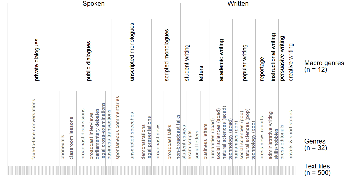
Now imagine that the corpus is divided into equal-sized chunks.
As a result, the meaning (and interpretation) of dispersion scores varies with the item’s corpus frequency. I would consider this problematic, because I agree with Egbert et al. (2020, 110), who note: “Dispersion results should always be interpreted and reported as ‘dispersion across _____’, where the blank is filled by the type of corpus unit across which dispersion was calculated”. For MB, the blank would need to be filled in differently depending on the corpus frequency of the item.
To see the range of interpretations we would need to attach to items in different frequency bands, I will rely on a set of 150 word forms, which was compiled by Biber et al. (2016) for methodological purposes, that is, to study the behavior of dispersion measures in different distributional settings. The items are intended to cover a broad range of frequency and dispersion levels. The dataset biber150_ice_gb in the {tlda} package includes text-level frequency information for these forms in ICE-GB (G. Nelson, Wallis, and Aarts 2002). Four items on Biber et al. (2016)’s list do not occur in ICE-GB (aye, corp, ltd, tt), leaving us with 146.
Figure 2 shows the (log-scaled) corpus frequency of the 146 items against three benchmarks: the number of macro genres (n = 12), genres (n = 32), and text files (n = 500). Divisions at the level of genres or macro genres are made for lower-frequency items with fewer than 50 occurrences (about a quarter of the word forms). Around half of the items have a corpus frequency greater than 500, and for these higher-frequency items, we would obtain measurements at or below the level of the text files in the corpus.
p1 <- histogram(
  log(rowSums(biber150_ice_gb_macro_genre[-1,])),
  par.settings = lattice_ls, axis = axis_bottom,
  col = "grey", breaks = seq(log(1), log(100000), length = 26) - 0.460517/2, ylim = c(0, 22),
  xlab = "Corpus frequency", ylab = "",
  scales = list(x = list(at = log(c(1, 10, 100, 1000, 10000, 100000)),
                         label = c("1", "10", "100", "1,000", "10,000", "100,000"))),
  panel = function(x,y,...){
    panel.segments(x0 = log(500), x1 = log(500), y0 = 0, y1 = 14, lty = "22", lineend = "butt")
    panel.segments(x0 = log(32), x1 = log(32), y0 = 0, y1 = 17, lty = "22", lineend = "butt")
    panel.segments(x0 = log(12), x1 = log(12), y0 = 0, y1 = 20, lty = "22", lineend = "butt")

    panel.text(x = log(500)-.15, y = 15.5, label = "Texts (n = 500)", adj = 0)
    panel.text(x = log(32)-.15, y = 18.5, label = "Genres (n = 32)", adj = 0)
    panel.text(x = log(12)-.15, y = 21.5, label = "Macro genres (n = 12)", adj = 0)

    panel.histogram(x, ...)
  })

print(p1, position = c(-.075, 0, .98, 1))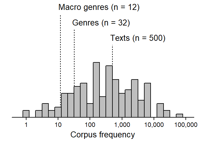
For many, myself included, it would be desirable to apply the Poissonness approach to an existing set of corpus parts, which ideally represent meaningful contexts of language use. This means that the measure should ideally also work with parts of different size. In this section, I describe a generalization of Nelson’s (2025) MB that meets these demands; I will label the resulting index DMB.
Before we go further, I should note that this requires us to abandon the virtue of computational simplicity. To calculate DMB, we need access to a statistical programming language such as R. For convenience, the measure can be computed with the function disp_DMB() in the R package {tlda} (Sönning 2025c).
Instead of using the simple approach proposed by R. N. Nelson (2025) (which, however, requires us to work with many different sets of arbitrary corpus chunks), we determine the expected proportion of empty parts using a Poisson regression model. In this model, the corpus parts constitute the individual observations, which are characterized by two counts:
The model itself does not include any predictor variables apart from what is referred to as an offset term, which gives the part sizes. This is necessary for the same reason we often calculate normalized frequencies: A frequency count (i.e. subfrequency) is only meaningful in relation to corpus size (i.e. part size). The regression model then allows us to estimate an intercept, which is \(\lambda\) (the average occurrence rate), expressed on the log scale. For a count regression model with an offset term, \(\lambda\) is the average occurrence rate (i.e. normalized frequency) per 1 word. For interpretation, the rate is expressed using a more appropriate basis (e.g. “per thousand/million words” instead of “per 1 word”).
Let us consider the implementation of this approach step by step. For illustration, we look at the dispersion of actually in ICE-GB, using the text files as corpus parts. We start by extracting the subfrequencies and part sizes from the data object biber150_ice_gb, which is part of the {tlda} package:
actually_subfreq <- biber150_ice_gb["actually",]
actually_partsize <- biber150_ice_gb["word_count",]
Then we specify a Poisson regression model with an offset term, using the base R function glm(). Note that part sizes are log-transformed before being passed to the function offset():
m <- glm(
  actually_subfreq ~ offset(log(actually_partsize)),
  family = poisson)
Let’s look at the regression table:
arm::display(m)glm(formula = actually_subfreq ~ offset(log(actually_partsize)),
family = poisson)
coef.est coef.se
(Intercept) -6.91 0.03
---
n = 500, k = 1
residual deviance = 1907.4, null deviance = 1907.4 (difference = 0.0)The model intercept, \(-6.91\), is the natural log occurrence rate per 1 word. To obtain an interpretable figure, we first exponentiate the intercept (to undo the loge-transformation):
exp(coef(m)) (Intercept)
0.0009949711 This amounts to a rate of about 0.001 per 1 word, which is better thought of as 1 per thousand words.
The next step is to obtain from the Poisson model the expected proportion of empty parts for the set of corpus parts that entered the analysis. It is important that this question be asked in this way, i.e. by reference to the set of parts in the data. This is because the probability of a part being empty or not primarily depends on its size. We therefore calculate the probability of a subfrequency of 0 for each part:
prob_0_all_parts <- dpois(
  0,
  exp(coef(m))*actually_partsize)
Then we take the average over these probabilities:
mean(prob_0_all_parts)[1] 0.1204614This is our Poisson-based estimate of \(\textrm{Pr}_{\textrm{exp}}(0)\). From here on, everything works in the same way as described by R. N. Nelson (2025). As an added benefit, we can use the regression model to produce approximate 95% confidence intervals.
The R function disp_DMB() carries out these computations:
disp_DMB(
  subfreq = actually_subfreq,
  partsize = actually_partsize,
  conf_int = TRUE,
  digits = 2,
  verbose = FALSE)
DMB ci_lower ci_upper
0.66 0.65 0.67 To compare the dispersion scores produced by MB and DMB, we turn to Biber et al. (2016)’s list of diagnostic items, and the ICE-GB corpus. Recall that ICE-GB only contains 146 out of the 150 items, so we work with this subset.
We start by calculating MB. What we need is the size of the corpus (1,072,393 tokens) and a data table that includes all occurrences of the 146 items in the corpus (here: 321,328 tokens in total). The data table must include a column that gives the corpus position for each occurrence. The following annotated code carries out the calculations.
# total number of token in ICE-GB
n_total <- 1072393

# data table with all occurrences of the 146 items including the corpus
# position of each occurrence
ice_gb_150_corpus_position <- readRDS("ice_gb_150_corpus_position.rds")

# create character vector listing all items
items <- unique(ice_gb_150_corpus_position$item)

# initiate vectors to store counts
freq_item <- NA
n_0 <- NA

# for each item, divide corpus into f parts, where f is the corpus frequency
# of the item and then count how many of these are empty
for(i in 1:length(items)){
  item_selected <- items[i]
  item_data <- subset(ice_gb_150_corpus_position, item == item_selected)
  freq_item[i] <- nrow(item_data)
  n_0[i] <- sum(table(cut(item_data$corpus_position, seq(0, n_total+1, length = nrow(item_data)+1))) == 0)
}

# combine results into data frame
ice_gb_150 <- data.frame(
  item = items,
  freq = freq_item,
  n_zeros = n_0
)

# add the observed proportion of empty parts
ice_gb_150$prop_zero <- ice_gb_150$n_zeros / ice_gb_150$freq

# calculate MB
ice_gb_150$MB <- ifelse(
  ice_gb_150$prop_zero <= exp(-1), 0,
  abs(ice_gb_150$prop_zero - exp(-1)) / (1 - exp(-1)))

# adjust to conventional scaling (0 = uneven; 1 = even)
ice_gb_150$MB <- 1 - ice_gb_150$MB
ice_gb_150 <- ice_gb_150[order(ice_gb_150$item),]
This gives us a data frame with the following columns:
item the item (146 in total)freq corpus frequencyn_zeros the number of empty partsprop_zero the proportion of empty parts (out of freq parts)MB the score for the dispersion measure MBstr(ice_gb_150)'data.frame': 146 obs. of 5 variables:
$ item : chr "a" "able" "actually" "after" ...
$ freq : int 20483 390 1067 871 364 181 4 2807 156 3198 ...
$ n_zeros : int 7752 175 608 378 195 127 3 1133 85 1276 ...
$ prop_zero: num 0.378 0.449 0.57 0.434 0.536 ...
$ MB : num 0.983 0.872 0.681 0.895 0.734 ...Next, we use the function disp_DMB() in the {tlda} package (Sönning 2025c) to calculate DMB. The text files will be used as corpus parts.
# initiate vector to store results
disp_scores_ice <- rep(NA, 150)

# loop through items and calculate DNB; for items with a corpus frequency
# of 0 (n = 4), the function returns NA
for(i in 1:150){
  if(sum(biber150_ice_gb[i+1,]) > 0){
      disp_scores_ice[i] <- disp_DMB(
        subfreq = biber150_ice_gb[i+1,],
        partsize = biber150_ice_gb[1,],
        print_score = FALSE,
        verbose = FALSE)
  }
}

# combine into a data frame
ice_gb_150_DMB <- data.frame(
  item = rownames(biber150_ice_gb)[-1],
  DMB = disp_scores_ice
)

# exclude items with a corpus frequency of 0 (where DMB is NA)
ice_gb_150_DMB <- subset(ice_gb_150_DMB, !is.na(DMB))

# combine with the data frame created above
ice_gb_150_nelson <- merge(ice_gb_150, ice_gb_150_DMB, by = "item")

# order alphabetically by item
ice_gb_150_nelson <- ice_gb_150_nelson[order(ice_gb_150_nelson$item),]
This adds one more column to the data frame:
DMB the score for the dispersion measure DMBstr(ice_gb_150_nelson)'data.frame': 146 obs. of 6 variables:
$ item : chr "a" "able" "actually" "after" ...
$ freq : int 20483 390 1067 871 364 181 4 2807 156 3198 ...
$ n_zeros : int 7752 175 608 378 195 127 3 1133 85 1276 ...
$ prop_zero: num 0.378 0.449 0.57 0.434 0.536 ...
$ MB : num 0.983 0.872 0.681 0.895 0.734 ...
$ DMB : num 1 0.84 0.657 0.861 0.744 ...We start by inspecting the overall distribution of MB and DMB scores using histograms. It is worth repeating here that I am expressing dispersion scores using the conventional scaling:
Figure 3 shows that the two measures yield a similar distribution, with scores pushing against the upper bound of the scale: For MB, only 14% of the items receive scores below .50, and for DMB this figure is at 12%. Considering the pool of items assembled by Biber et al. (2016), which aim to cover a broad range of frequency and dispersion levels, it seems that both measures show a bias toward evenness.
p1 <- histogram(
  ~ MB, data = ice_gb_150_nelson,
  xlim = c(0,1), ylim = c(0, 20),
  breaks = seq(0, 1, .05),  col = "grey",
  scales = list(x = list(at = c(0, 1),
                         label = c("0\n(uneven)", "1\n(even)"))),
  ylab = NULL, xlab = NULL, xlab.top = expression(MB),
  par.settings = lattice_ls, axis = axis_bottom)

p2 <- histogram(
  ~ DMB, data = ice_gb_150_nelson,
  xlim = c(0,1), ylim = c(0, 20),
  breaks = seq(0, 1, .05),  col = "grey",
  scales = list(x = list(at = c(0, 1),
                         label = c("0\n(uneven)", "1\n(even)"))),
  ylab = NULL, xlab = NULL, xlab.top = expression(D[MB]),
  par.settings = lattice_ls, axis = axis_bottom)

cowplot::plot_grid(NULL, p1, NULL, p2, NULL,
                   nrow = 1, rel_widths = c(-.1, 1, .1, 1, .07))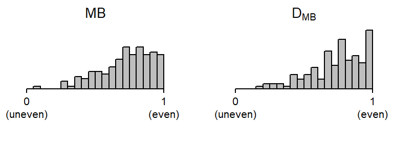
Let’s also look at the relationship between these measures and frequency. Figure 4 again shows similar constellations. What is particularly noteworthy for both MB and DMB is that they show no notable association with frequency. This is in stark contrast to other parts-based dispersion measures, which show a very strong, spurious correlation with frequency. In fact, this has emerged as one of the most important weaknesses of existing parts-based dispersion measures, and it has spawned methodological efforts to remove the unwanted influence that frequency has on dispersion scores (see Gries 2022, 2024). The fact that MB and DMB appear to measure dispersion independently from frequency is an attractive feature of these measures.
p1 <- xyplot(
  MB ~ log(freq), data = ice_gb_150_nelson, ylim = c(0,1),
  xlab = "Frequency (log-scaled)", ylab = "\n\nDispersion",
  scales = list(
    x = list(at = log(c(1,10,100, 1000, 10000)),
             label = c(1,10,100, 1000, 10000)),
    y = list(at = c(0, 1),
             label = c("\n0\n(uneven)", "(even)\n1\n"))),
  par.settings = lattice_ls, axis = axis_L,
  panel = function(x,y,...){
    panel.points(x,y,...)
    panel.text(x = log(300), y = 1.15, label = "MB")
  })

p2 <- xyplot(
  DMB ~ log(freq), data = ice_gb_150_nelson, ylim = c(0,1),
  xlab = "Frequency (log-scaled)", ylab = "",
  scales = list(
    x = list(at = log(c(1,10,100, 1000, 10000)),
             label = c(1,10,100, 1000, 10000)),
    y = list(at = c(0, 1))),
  par.settings = lattice_ls, axis = axis_L,
  panel = function(x,y,...){
    panel.points(x,y,...)
    panel.text(x = log(300), y = 1.15, label = expression(D[MB]))
  })

cowplot::plot_grid(
  NULL, NULL, NULL,
  NULL, p1, p2,
  nrow = 2,
  rel_widths = c(-.08, 1.1, 1),
  rel_heights = c(.125, 1))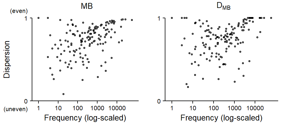
Let us finally compare the MB and DMB values we obtain for each item directly. To this end, Figure 5 graphs these scores against one another. The grey diagonal line represents identity, i.e. perfect agreement between MB and DMB; indeed most items fall near this line. Items above the diagonal (e.g. aha, da, bloke, nodded) receive higher dispersion scores from DMB, meaning that DMB suggests that they are more evenly distributed than MB. For items below the diagonal (e.g. minus, charles, percent), MB suggests greater evenness.
p1 <- xyplot(
  DMB ~ MB, data = ice_gb_150_nelson, xlim = c(0, 1), ylim = c(0, 1),
  ylab = expression(D[MB]), xlab = "MB", axis = axis_L,
  scales = list(
    x = list(at = c(0, 1)),
    y = list(at = c(0, 1))),       par.settings = lattice_ls,
  panel = function(x,y){
    panel.abline(a = 0, b = 1, col = "grey")
    panel.text(x, y, label = as.character(ice_gb_150_nelson$item),
               cex = .8, fontface = "italic")
  })

print(p1, position = c(0,0,.96, 1))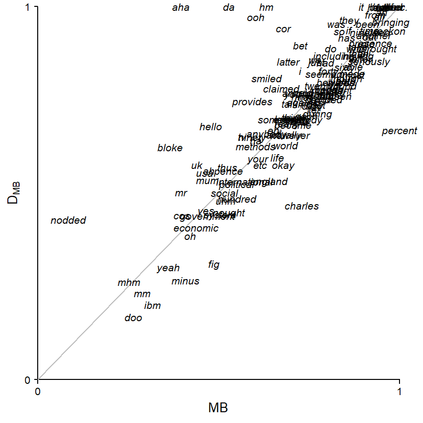
Let’s take a closer look at some items to see why the two measures yield different scores. For aha, which occurs 4 times in the corpus, MB produces a lower score (.40 vs. 1):
subset(ice_gb_150_nelson, item == "aha") item freq n_zeros prop_zero MB DMB
7 aha 4 3 0.75 0.3954942 1This is because, upon dividing ICE-GB into four equal-sized parts, aha appears in only one of them, and a distribution of 0 0 0 4 is quite uneven. This reflects the fact that aha only occurs in the spoken part. Since MB divides the corpus into few chunks, its score for this item reflects its association with spoken registers. DMB, on the other hand, returns a score of 1, because the four occurrences stem from different texts (i.e. corpus parts). This means that, at this level of analysis (500 corpus parts, i.e. text files), the four occurrences are distributed as evenly as possible – each in a different text.
table(biber150_ice_gb["aha",])
  0   1
496   4
For percent, MB yields a higher score (1 vs. .67), suggesting greater evenness. Upon dividing the corpus into three parts, one part is empty, which aligns with the expectations based on the Poisson distribution. The meaning of this score is somewhat unclear. Reference back to Figure 1 shows that a division of ICE-GB into thirds yields a spoken, a written, and a mixed part, which obscures the meaning carried by the score.
subset(ice_gb_150_nelson, item == "percent") item freq n_zeros prop_zero MB DMB
102 percent 3 1 0.3333333 1 0.6686852DMB gives a lower score to percent. This is because an even distribution would have seen the three instances of percent spread across three different parts (i.e. text files). However, one text contains two occurrences of the item:
table(biber150_ice_gb["percent",])
  0   1   2
498 1 1 In this blog post, I have described how R. N. Nelson (2025)’s MB can be extended to work with a pre-determined set of corpus parts that may differ in size. The resulting measure DMB is implemented in the R function disp_DMB() in the {tlda} package. In my view, this modification of MB overcomes what I would consider a major concern with MB: Its reliance on equal-sized corpus parts whose number varies across items.
To summarize our examination of MB and DMB, we may note the following pros and cons:
R. N. Nelson (2025) provides new and welcome impulses for methodological research on the measurement of dispersion. It may be too early, however, to conclude that MB may be considered “a measure with generally superior performance” (R. N. Nelson 2025, 121).
However, computational cost arises at the stage of data preparation: for each item, the corpus needs to be divided anew, into f parts.↩︎
@online{sönning2025,
  author = {Sönning, Lukas},
  title = {Nelson’s (2025) {Poisson-based} Dispersion Measure},
  date = {2025-10-30},
  url = {https://lsoenning.github.io/posts/2025-10-23_dispersion_nelson_poissonness/},
  langid = {en}
}