PhD workshop

Session 2: Data import/export and data visualization

Getting data into R

Data and R: Warnings

• Importing data into R can be frustrating
• Getting them into shape for analysis is often tedious

Data preparation: General workflow

• Data entry/annotation usually in MS Excel
• Store Excel spreadsheet in subfolder data/input_data
• Load into R (document this step in code form)
• Prepare for analysis
• Save in .tsv format in subfolder data/analysis_data

Reproducibility

The .tsv format ensures that your data can be opened using other software (interoperability).

Download data

• Create subfolders:
  • data/input_data
  • data/analysis_data
• Download data files from https://osf.io/j43v9/
  • data_quantifiers.tsv
  • data_quantifiers_wide.xlsx
• Save them in subfolder data/input_data

Data preparation: Simple rules

• Lots of work can be avoided by following a few simple rules
• Rows and columns
  • Columns are variables
  • Rows are observations
  • Avoid blank rows and blank columns
  • The first row gives the name of the variables

Learn more about data preparation in spreadsheets

Data preparation: Naming conventions

• Avoid blank spaces and special symbols (underscore _ is OK)
• Do not begin variable names with numbers
• R is case-sensitive (“Yes” and “yes” are treated as different)
• Code missing values (empty cells) as NA

Errors

A lot can go wrong when reading data into R. Make sure you routinely include error checks into your workflow. Always carefully inspect the data at different stages of processing/analysis.

Working with data tables

Data import

• Different functions for different file formats
• Most typical formats
  • .xlsx read_excel() (package: readxl)
  • .csv read.csv() or read.csv2()
  • .txt read.delim()
  • .tsv read_tsv() (package: tidyverse)

Helpful button: “Import dataset”

• Use the button “Import dataset”
• Problem: Point-and-click commands not reproducible
• Solution: Copy-and-paste the generated R code into your notebook
• Change name of data frame: d
• Change directory path: Use here()

Import Excel spreadsheets

Packages

• Load packages {readxl} and {here}
• If they are not installed yet, do so first: install.packages()

library(readxl)
library(here)

Using here() to locate files

• here("directory", "file_name")
• Root (where path begins) = project directory
• Find root

here()

[1] "C:/Users/ba4rh5/Work Folders/My Files/R projects/teaching/phd_workshop"

Read in Excel file

• Function: read_xlsx()
• Use assignment operator (Alt + -)
• Should appear in workspace

d <- read_xlsx(
    here("data/input_data", 
         "data_quantifiers_wide.xlsx"))

Inspect data frame

• Look at contents

str(d)

• Inspect first few rows:

head(d)

Import .tsv file

Read in .tsv file

• Function: read_tsv() (part of the tidyverse)

library(tidyverse)

d <- read_tsv(
    here("data/input_data",
         "data_quantifiers.tsv"))

Learn more about reading in different kinds of data: Wickham & Grolemund 2023: Chapter 11

Inspect data frame

str(d)

spc_tbl_ [80 x 3] (S3: spec_tbl_df/tbl_df/tbl/data.frame)
 $ subject   : chr [1:80] "subj_01" "subj_02" "subj_03" "subj_04" ...
 $ quantifier: chr [1:80] "few" "few" "few" "few" ...
 $ percent   : num [1:80] 5 20 10 8 12 15 25 10 15 10 ...
 - attr(*, "spec")=
  .. cols(
  ..   subject = col_character(),
  ..   quantifier = col_character(),
  ..   percent = col_double()
  .. )
 - attr(*, "problems")=<externalptr> 

Look at the first rows of a data frame: head()

head(d)

# A tibble: 6 x 3
  subject quantifier percent
  <chr>   <chr>        <dbl>
1 subj_01 few              5
2 subj_02 few             20
3 subj_03 few             10
4 subj_04 few              8
5 subj_05 few             12
6 subj_06 few             15

Use $ to access a column (variable) in the data frame

d$percent

 [1]  5.0 20.0 10.0  8.0 12.0 15.0 25.0 10.0 15.0 10.0 10.0 10.0  7.0 15.0 15.0
[16]  6.0  5.0 10.0 15.0 10.0 15.0 35.0 27.5 20.0 30.0 35.0 40.0 30.0 33.0 33.0
[31] 25.0 40.0 20.0 40.0 30.0 14.0 12.5 25.0 40.0 20.0 30.0 70.0 65.0 51.0 50.0
[46] 60.0 67.5 60.0 67.0 67.0 50.0 70.0 60.0 69.0 75.0 75.0 65.0 70.0 75.0 80.0
[61] 50.0 80.0 85.0 80.0 75.0 90.0 92.5 80.0 85.0 90.0 75.0 90.0 85.0 90.0 85.0
[76] 91.0 80.0 90.0 90.0 90.0

Write a data table to file: write_tsv()

write_tsv(
    d,
    here("data(/analysis_data", 
         "data_quantifiers.txt"))

Saving data tables

To make sure you never overwrite the input data file, keep the input data in the subfolder data/input_data, and the processed data in the subfolder data/analysis_data.

Working with data

The dplyr package

• Use the dplyr package (part of the tidyverse)
• General approach: Piping
  • Pipe operator |> or %>%
  • Keyboard shortcut: Ctrl + Shift + M
• Perform a sequence (pipeline) of operations on data frames

dplyr functions

• filter() Select a subset of observations
• select() Select a subset of variables
• arrange() Change order of rows based on a variable
• mutate() Add new variables that are functions of data in the table
• summarize() Obtain data summaries (mean, count, sd, etc.)
• group_by() Form groups

Learn more: Wickham & Grolemund 2023: Chapter 4, Chapter 5 | Vignettes for the dplyr package

Select a subset of observations: filter()

• Specify subset based on levels/values of a variable
• In R, “is equal to” is ==

d |> filter(subject == "subj_01")

# A tibble: 4 x 3
  subject quantifier percent
  <chr>   <chr>        <dbl>
1 subj_01 few              5
2 subj_01 some            15
3 subj_01 many            30
4 subj_01 most            50

Select a subset of variables: select()

d |> select(subject, percent)

# A tibble: 80 x 2
   subject percent
   <chr>     <dbl>
 1 subj_01       5
 2 subj_02      20
 3 subj_03      10
 4 subj_04       8
 5 subj_05      12
 6 subj_06      15
 7 subj_07      25
 8 subj_08      10
 9 subj_09      15
10 subj_10      10
# i 70 more rows

Reorder rows based on a variable: arrange()

d |> arrange(quantifier)

# A tibble: 80 x 3
   subject quantifier percent
   <chr>   <chr>        <dbl>
 1 subj_01 few              5
 2 subj_02 few             20
 3 subj_03 few             10
 4 subj_04 few              8
 5 subj_05 few             12
 6 subj_06 few             15
 7 subj_07 few             25
 8 subj_08 few             10
 9 subj_09 few             15
10 subj_10 few             10
# i 70 more rows

Data summary: group_by() and summarize()

• Obtain data summaries (mean, count, sd, etc.)

d |> group_by(subject) |> 
    summarize(
        mean_percent = mean(percent))

# A tibble: 20 x 2
   subject mean_percent
   <chr>          <dbl>
 1 subj_01         25  
 2 subj_02         51.2
 3 subj_03         46.9
 4 subj_04         39.8
 5 subj_05         41.8
 6 subj_06         50  
 7 subj_07         56.2
 8 subj_08         45  
 9 subj_09         50  
10 subj_10         50  
11 subj_11         40  
12 subj_12         52.5
13 subj_13         43  
14 subj_14         53.5
15 subj_15         51.2
16 subj_16         46.5
17 subj_17         40.6
18 subj_18         48.8
19 subj_19         55  
20 subj_20         50  

dplyr functions: Longer pipes

• Mean percentage by subject: group_by() and summarize()

d |> group_by(subject) |> 
    summarize(
        mean_percent = mean(percent))

# A tibble: 20 x 2
   subject mean_percent
   <chr>          <dbl>
 1 subj_01         25  
 2 subj_02         51.2
 3 subj_03         46.9
 4 subj_04         39.8
 5 subj_05         41.8
 6 subj_06         50  
 7 subj_07         56.2
 8 subj_08         45  
 9 subj_09         50  
10 subj_10         50  
11 subj_11         40  
12 subj_12         52.5
13 subj_13         43  
14 subj_14         53.5
15 subj_15         51.2
16 subj_16         46.5
17 subj_17         40.6
18 subj_18         48.8
19 subj_19         55  
20 subj_20         50  

dplyr functions: Longer pipes

• Sort subjects by mean percentage: arrange()

d |> group_by(subject) |> 
    summarize(
        mean_percent = mean(percent)) |> 
    arrange(mean_percent)

# A tibble: 20 x 2
   subject mean_percent
   <chr>          <dbl>
 1 subj_01         25  
 2 subj_04         39.8
 3 subj_11         40  
 4 subj_17         40.6
 5 subj_05         41.8
 6 subj_13         43  
 7 subj_08         45  
 8 subj_16         46.5
 9 subj_03         46.9
10 subj_18         48.8
11 subj_06         50  
12 subj_09         50  
13 subj_10         50  
14 subj_20         50  
15 subj_02         51.2
16 subj_15         51.2
17 subj_12         52.5
18 subj_14         53.5
19 subj_19         55  
20 subj_07         56.2

dplyr functions: Longer pipes

• We want to sort in descending order: desc(...)

d |> group_by(subject) |> 
    summarize(
        mean_percent = mean(percent)) |> 
    arrange(desc(mean_percent))

# A tibble: 20 x 2
   subject mean_percent
   <chr>          <dbl>
 1 subj_07         56.2
 2 subj_19         55  
 3 subj_14         53.5
 4 subj_12         52.5
 5 subj_02         51.2
 6 subj_15         51.2
 7 subj_06         50  
 8 subj_09         50  
 9 subj_10         50  
10 subj_20         50  
11 subj_18         48.8
12 subj_03         46.9
13 subj_16         46.5
14 subj_08         45  
15 subj_13         43  
16 subj_05         41.8
17 subj_17         40.6
18 subj_11         40  
19 subj_04         39.8
20 subj_01         25  

dplyr functions: Longer pipes

• Only subjects with below 40%: filter()

d |> group_by(subject) |> 
    summarize(
        mean_percent = mean(percent)) |> 
    arrange(desc(mean_percent)) |> 
    filter(mean_percent <= 40)

# A tibble: 3 x 2
  subject mean_percent
  <chr>          <dbl>
1 subj_11         40  
2 subj_04         39.8
3 subj_01         25  

Data visualization

Data visualization: Resources

• Use the ggplot2 package (part of the tidyverse)
• Healy 2017
• Wickham & Grolemund 2023: Chapter 3 (free online)
• Chang 2023 (free online)

ggplot2

The way in which ggplot2 works may seem confusing at first. However, it is a very flexible and powerful tool and has become the de-facto standard for adanced data visualization in R. There is a large community of users, which makes it easy to find help online.

Data visualization: Disagreement data

• Obtain distribution of percentage means across subjects

d |> group_by(subject) |> 
    summarize(
        mean_percent = mean(percent))

# A tibble: 20 x 2
   subject mean_percent
   <chr>          <dbl>
 1 subj_01         25  
 2 subj_02         51.2
 3 subj_03         46.9
 4 subj_04         39.8
 5 subj_05         41.8
 6 subj_06         50  
 7 subj_07         56.2
 8 subj_08         45  
 9 subj_09         50  
10 subj_10         50  
11 subj_11         40  
12 subj_12         52.5
13 subj_13         43  
14 subj_14         53.5
15 subj_15         51.2
16 subj_16         46.5
17 subj_17         40.6
18 subj_18         48.8
19 subj_19         55  
20 subj_20         50  

Data visualization: Disagreement data

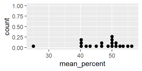
• Visualize using a dot diagram

d |> group_by(subject) |> 
    summarize(
        mean_percent = mean(percent)) |> 
    ggplot(aes(x = mean_percent)) +
    geom_dotplot(binwidth = 1)

Saving graphics

• Use ggsave() to save graph as PDF
• Use here() to refer to subfolder “figures”

ggsave(
  here("figures", 
       "mean_percentage_by_subject.pdf"), 
  width = 3, 
  height = 1.5)

Saving graphs: File format

Always save graphs as PDF files, to have publication-quality images. If you need to insert a graph into a PowerPoint (or Word), use the free software IrfanView: (1) Open the PDF using Adobe Acrobat, (2) Zoom in/out to set the resolution, (3) Make a screenshot, (4) Paste it (Ctrl. + V) into IrfanView, (5) cut out the graph (Ctrl. + C), and (6) paste it (Ctrl. + V) into PowerPoint/Word.

ggplot2: Dot plot

d |> group_by(subject) |> 
    summarize(
        mean_percent = mean(percent)) |> 
    ggplot(aes(x = mean_percent,
               y = subject)) +
    geom_point()

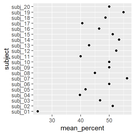
ggplot2: Dot plot

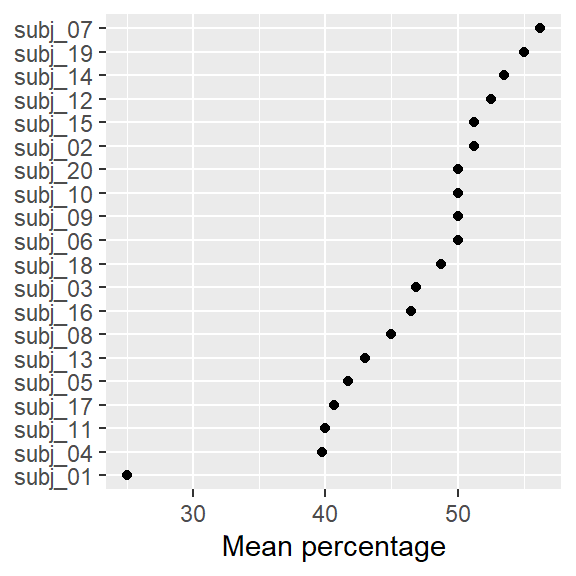
• Order

d |> group_by(subject) |> 
    summarize(
        mean_percent = mean(percent)) |> 
    ggplot(aes(x = mean_percent,
               y = reorder(subject, mean_percent))) +
    geom_point()

ggplot2: Dot plot

• Change axis labels

d |> group_by(subject) |> 
    summarize(
        mean_percent = mean(percent)) |> 
    ggplot(aes(x = mean_percent,
               y = reorder(subject, mean_percent))) +
    geom_point() +
    xlab("Mean percentage") +
    ylab(NULL)

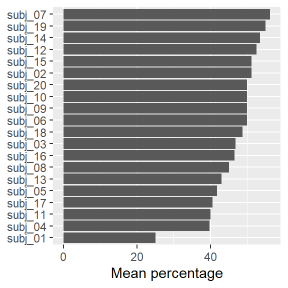
ggplot2: Dot plot

• Change into bar chart

d |> group_by(subject) |> 
    summarize(
        mean_percent = mean(percent)) |> 
    ggplot(aes(x = mean_percent,
               y = reorder(subject, mean_percent))) +
    geom_col() +
    xlab("Mean percentage") +
    ylab(NULL)