PhD workshop

Session 1: R project setup and Quarto documents

In general

  • Use R with RStudio
  • Create an RStudio project for each new research project/study
  • Use analysis notebooks (Quarto documents), which include R code + output
  • Project folder: Organization into subfolders (data, figures, etc.)
  • Everything should always be reproducible from code + input data

R projects: Setup

Create an RStudio project

  • File : New project…
  • New Directory
  • New Project
  • Use an informative directory name
  • Store it where you will find it

RStudio project organization

  • A project should be self-contained: All in one place
  • Keep data files and analysis notebooks in your project folder
  • Use subfolders: data, figures

Reproducibility

Your data analysis project should be self-contained, which means that everything that is needed to reproduce the results is stored in the project folder.

RStudio project setup

  • Go to your project folder
  • Create two subfolders: data, figures

Quarto documents

Use analysis notebooks (Quarto documents)

  • Quarto documents combine text, code, and output
  • Can be exported as html/Word/PDF file
  • In the analysis notebook:
    • Talk to your (future) self: Say what you do (and why you do it)
    • Run analyses
    • Look at output (figures, tables,…)

Create a Quarto document

  • File : New file : Quarto document…
  • Use default options, click “Create”
  • Save it in your project folder
  • Render it: Click the Render button

Play around with the Quarto file

  • Compare contents of file with rendered version
  • Change/add text and render again
  • Add headers / sub-headers
  • Run code inside of RMarkdown file
  • Add bold print **bold**
  • Add italics *italics*
  • Have a look at the RMarkdown Cheat Sheet

R basics

R: General advice

  • Use the tidyverse set of packages
  • Use ggplot2 for data visualization (Session 2)
  • Workflow: Document every step using code
  • Aim: Full reproducibility based on code + data

R packages

  • For some things, you need packages (sets of functions)
  • You need to install a package only once: install.packages()
install.packages("tidyverse")
  • Packages must be loaded at beginning of R session: library()
library(tidyverse)
  • Notebooks should start with section ## R setup, where you load the packages you need

In R, everything is an object

  • Functions, data tables, etc.
  • Create an object by assigning something to a new name
  • Assignment operator: <- (shortcut: Alt + -)
  • New objects then exist in R’s workspace (top right panel)
  • Important object types:
    • Vector: Sequence of elements (e.g. names, numbers)
    • Data frame/tibble: Data tables

In R, you do things using functions

  • Functions do the work in R (calculation, graphing, etc.)
  • Functions have parentheses at the end of their names
  • We give instructions to a function using its arguments
  • function(argument = "...")

Some useful functions

  • Inspect contents of data frame: str()
  • Inspect first few rows of data frame: head()
  • mean(), median()

Action: Explore PhDPublications dataset

Get data

  • Install and load AER package (that’s where the data is)
install.packages("AER")
library(AER)
  • Run following code to be able to use the data set:
data(PhDPublications)
  • Dataset appears as an object in your workspace (top right panel)

Save typing

  • Assign data frame to a new object called d (= copy it)
  • Assignment operator:
    • <-
    • shortcut: Alt + - (Mac: Option + -)
d <- PhDPublications
  • RStudio also also offers code completion: Tab key
  • Try it: Type Ph and hit Tab key

Inspect contents of data frame

  • Contents: str()
  • Look at first few rows: head()

Inspect contents of data frame

  • Variables
    • articles # articles published during last 3 years of PhD
    • gender
    • married
    • kids # of children less than 6 years old
    • prestige prestige of graduate program
    • mentor # articles published by mentor

Inspect contents of data frame

'data.frame':   915 obs. of  6 variables:
 $ articles: int  0 0 0 0 0 0 0 0 0 0 ...
 $ gender  : Factor w/ 2 levels "male","female": 1 2 2 1 2 2 2 1 1 2 ...
 $ married : Factor w/ 2 levels "no","yes": 2 1 1 2 1 2 1 2 1 2 ...
 $ kids    : int  0 0 0 1 0 2 0 2 0 0 ...
 $ prestige: num  2.52 2.05 3.75 1.18 3.75 ...
 $ mentor  : int  7 6 6 3 26 2 3 4 6 0 ...
 - attr(*, "datalabel")= chr "Academic Biochemists / S Long"
 - attr(*, "time.stamp")= chr "30 Jan 2001 10:49"
 - attr(*, "formats")= chr [1:6] "%9.0g" "%9.0g" "%9.0g" "%9.0g" ...
 - attr(*, "types")= int [1:6] 98 98 98 98 102 98
 - attr(*, "val.labels")= chr [1:6] "" "sexlbl" "marlbl" "" ...
 - attr(*, "var.labels")= chr [1:6] "Articles in last 3 yrs of PhD" "Gender: 1=female 0=male" "Married: 1=yes 0=no" "Number of children < 6" ...
 - attr(*, "version")= int 6
 - attr(*, "label.table")=List of 6
  ..$ marlbl: Named num [1:2] 0 1
  .. ..- attr(*, "names")= chr [1:2] "Single" "Married"
  ..$ sexlbl: Named num [1:2] 0 1
  .. ..- attr(*, "names")= chr [1:2] "Men" "Women"
  ..$       : NULL
  ..$       : NULL
  ..$       : NULL
  ..$       : NULL

Structure your Quarto document

  • Use headings
    • ### R setup (load packages)
    • ### Data (load data)
    • ### Descriptive analysis (tables, graphs)
  • Keyboard shortcut to insert code chunk:
    • Ctrl + Alt + I (Mac: Command + Option + I)

Create tables

R package: dplyr

  • Part of the tidyverse
  • Piping
    • |>
    • Means “and then”
    • Shortcut: Strg + Shift + M (Mac: Cmd + Shift + M)

How many male and female PhD students?

  • Useful functions
    • group_by() divide the dataset
    • summarize() summarize subsets
    • n() count how many there are
d |>
  group_by(gender) |> 
  summarise(
    N = n())
# A tibble: 2 x 2
  gender     N
  <fct>  <int>
1 male     494
2 female   421

Task

  • Create tables to answer the following questions
  • How many PhD students…
    • … are married?
    • … have no kids?

Number of articles by kid count

  • mean(), median(), sd(), max()
d |> 
  group_by(kids) |> 
  summarise(
    N = n(),
    mean_pubs = mean(articles),
    median_pubs = median(articles),
    sd_pubs = sd(articles),
    max_pubs = max(articles))
# A tibble: 4 x 6
   kids     N mean_pubs median_pubs sd_pubs max_pubs
  <int> <int>     <dbl>       <dbl>   <dbl>    <int>
1     0   599     1.72            1   1.93        19
2     1   195     1.76            1   2.05        12
3     2   105     1.54            1   1.74        11
4     3    16     0.812           1   0.911        3

Create graphs

R package ggplot2

  • Part of the tidyverse
  • “Grammar of Graphics”

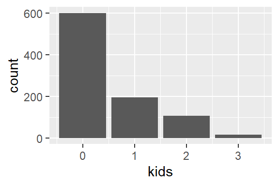
How many PhD students have (how many) kids?

d |> ggplot(aes(x = kids)) + 
    geom_bar()

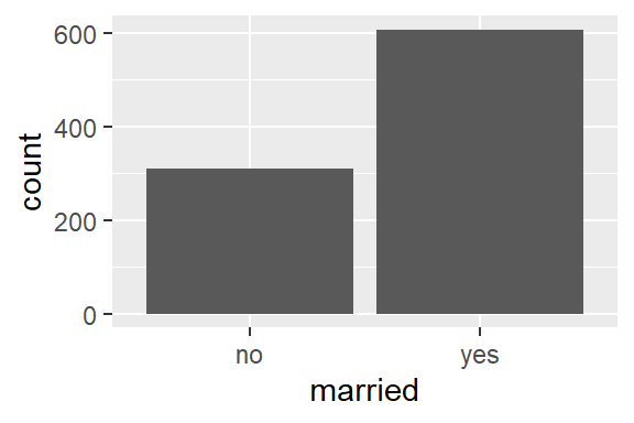
How many PhD students are married?

d |> ggplot(aes(x = married)) + 
    geom_bar()

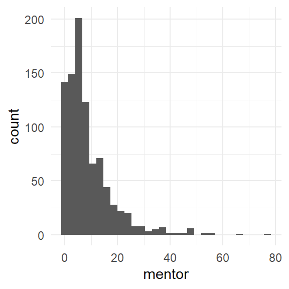
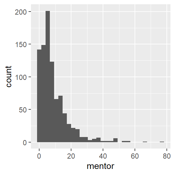
Distribution: Number of articles by mentor

d |> ggplot(aes(x = mentor)) + 
    geom_histogram()

Explore themes

d |> ggplot(aes(x = mentor)) + 
    geom_histogram() +
    theme_minimal()